geosnap and geoprocessing

Geosnap

geosnap - the geospatial neighborhood analysis package - provides a suite of tools for understanding the composition and extent of [endogenous] neighborhoods and regions in a study area. It provides:

• simple access to commonly-used datasets in urban and regional analyses:
  • demographic data (Census/ACS)
  • employment (LEHD)
  • environment (EPA)
  • travel infrastructure (OSM)
  • public education systems (NCES)
• an easy interface to build geodemographic typologies
  • classic aspatial typologies
  • constrained homogenous regions
• built-in functionality to facilitate spatiotemporal analysis
  • within time-period standardization
  • boundary harmonization
  • inflation adjustment
• bespoke plotting tools to help visualize neighborhood dynamics
  • temporally-static choropleth mapping
  • animated mapping
• state-of-the-art techniques for modeling neighborhood change over time
  • spatial Markov transition models
  • sequence analysis

Today, we want to focus on getting data from geosnap. This involves two basic steps: instantiate a DataStore class which points to datasets installed on the 385 course server, then querying the new DataStore object using functions from the geosnap io (for input-ouput) module

import geopandas as gpd
import pandas as pd
import geosnap
geosnap.__version__

'0.14.0'

from geosnap import DataStore

All of the datasets available in geosnap can be streamed from the cloud or installed on a local machine for analysis. In many cases, streaming works fine, but for repeated use of the same datasets, it is easier to install the data permanently. We have already done that on the course server. To ensure geosnap can access that data, we instantiate a new DataStore object pointing to the location of the data

datasets = DataStore("/srv/data/geosnap")

The datasets object can now be used to read and write data from the "/srv/data/geosnap/" folder, which is where the course data lives).

As a quick shorthand to see the available datasets, you can use the dir function to peek inside the datasets object

dir(datasets)

['acs',
 'bea_regions',
 'blocks_2000',
 'blocks_2010',
 'blocks_2020',
 'codebook',
 'counties',
 'ejscreen',
 'lodes_codebook',
 'ltdb',
 'msa_definitions',
 'msas',
 'ncdb',
 'nces',
 'seda',
 'show_data_dir',
 'states',
 'tracts_1990',
 'tracts_2000',
 'tracts_2010',
 'tracts_2020']

Each of these is a dataset that can be accessed. For more information on the datasets, see the geosnap datasets page.

As one example, we can collect data from the U.S. Census American Community Survey (5-year survey estimates) using the get_acs function in geosnap’s io module.

from geosnap import io as gio

First we import the io module, aliased as gio, then we query the DataStore (called datasets) for ACS data at the tract level for state 06 (which is California) and year 2016 (which is the 2012-2016 ACS).

Census Data

from geosnap.io import get_acs

ca = get_acs(datasets, state_fips=['06'], level='tract', years=[2016])

/home/serge/miniforge3/envs/workshop-pysal/lib/python3.10/site-packages/geosnap/_data.py:16: UserWarning: Streaming data from S3. Use `geosnap.io.store_acs()` to store the data locally for better performance
  warn(warning_msg)

The ca variable now holds a geodataframe of California census data at the tract level. To get a different year or a different geographic level, we could specify different input parameters to the get_acs function

ca.head()

	geoid	n_mexican_pop	n_cuban_pop	n_puerto_rican_pop	n_russian_pop	n_italian_pop	n_german_pop	n_irish_pop	n_scandaniavian_pop	n_foreign_born_pop	...	p_poverty_rate	p_poverty_rate_over_65	p_poverty_rate_children	p_poverty_rate_white	p_poverty_rate_black	p_poverty_rate_hispanic	p_poverty_rate_native	p_poverty_rate_asian	geometry	year
0	06001400100	55.0	0.0	13.0	49.0	62.0	147.0	13.0	8.0	843.0	...	3.752906	0.531385	0.631020	3.055463	0.000000	0.000000	0.0	0.000000	MULTIPOLYGON (((-122.24692 37.88544, -122.2466...	2016
1	06001400200	118.0	0.0	25.0	17.0	39.0	57.0	26.0	6.0	243.0	...	5.430328	1.946721	0.000000	4.047131	0.000000	0.563525	0.0	0.000000	MULTIPOLYGON (((-122.25792 37.84261, -122.2577...	2016
2	06001400300	171.0	0.0	0.0	0.0	154.0	81.0	75.0	0.0	857.0	...	8.732777	1.765962	0.329905	3.299049	3.648360	0.426936	0.0	0.000000	MULTIPOLYGON (((-122.26563 37.83764, -122.2655...	2016
3	06001400400	127.0	9.0	0.0	56.0	55.0	84.0	37.0	0.0	471.0	...	6.445406	0.721501	0.000000	3.799904	0.673401	0.553151	0.0	0.000000	MULTIPOLYGON (((-122.26183 37.84162, -122.2618...	2016
4	06001400500	282.0	29.0	11.0	10.0	7.0	103.0	51.0	0.0	635.0	...	9.081168	0.375033	0.000000	4.178945	3.375301	3.402089	0.0	0.642915	MULTIPOLYGON (((-122.26951 37.84858, -122.2693...	2016

5 rows × 158 columns

ca.plot()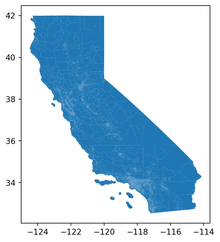

To trim down the existing dataset, for example to “slice out” the tracts in San Diego county, we use pandas dataframe operations. Here we use the geoid column to select tracts that begin with “06073”, which is the county FIPS code for San Diego

sd = ca[ca.geoid.str.startswith('06073')]

sd.plot()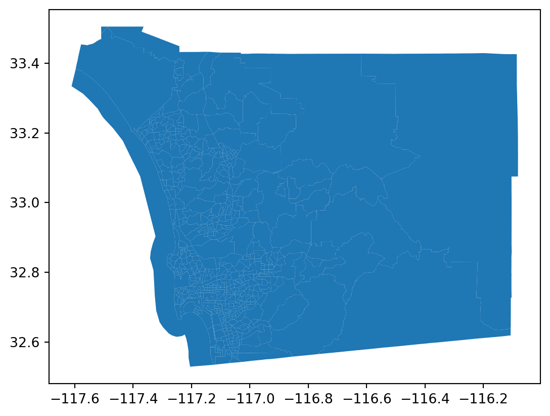

EPA Environmental Justice Screening Data

The Environmental Protection Agency (EPA)’s envrironmental justice screening tool (EJSCREEN) is a national dataset that provides a wealth of environmental (and some demographic) data at a blockgroup level. For a full list of indicators and their metadata, see the EPA page, but this dataset includes important variables like air toxics cancer risk,ozone concentration in the air, particulate matter, and proximity to superfund sites.

The EJSCREEN data can be queried similarly to the ACS data. For example to get blockgroup-level data for the Seattle metropolitan region in 2019, we would use the following

sea_ejscreen = gio.get_ejscreen(datasets, msa_fips="42660", years=2019).to_crs(4326)

/home/serge/miniforge3/envs/workshop-pysal/lib/python3.10/site-packages/geosnap/_data.py:16: UserWarning: Streaming data from S3. Use `geosnap.io.store_ejscreen()` to store the data locally for better performance
  warn(warning_msg)

A description of the variables in the EJSCREEN data is available here. A subset of the interesting variables we might examine is provided in the table below

Variable	Description
DSLPM	Diesel particulate matter level in air
CANCER	Air toxics cancer risk
RESP	Air toxics respiratory hazard index
PTRAF	Traffic proximity and volume
PWDIS	Indicator for major direct dischargers to water
PNPL	Proximity to National Priorities List (NPL) sites
PRMP	Proximity to Risk Management Plan (RMP) facilities
PTSDF	Proximity to Treatment Storage and Disposal (TSDF) facilities
OZONE	Ozone level in air
PM25	PM2.5 level in air

sea_ejscreen.plot()

Geoprocessing

Once a dataset is selected, we often need to perform more transformations and data operations than can be performed via table operations. That is, we often want to use the spatial information stored in each observation as a way of transforming, subsetting, aggregating, or otherwise manipulating the data.

These kinds of operations that rely on geospatial information are often called geoprocessing operations, and in this notebook we cover a subset of geoprocessing methods:

• Coordinate reference system transformations
• Spatial joins
• Spatial aggregations

sea_ejscreen.head()

	geoid	ACSTOTPOP	ACSIPOVBAS	ACSEDUCBAS	ACSTOTHH	ACSTOTHU	MINORPOP	MINORPCT	LOWINCOME	LOWINCPCT	...	T_PM25_P2	T_PM25_P6	AREALAND	AREAWATER	NPL_CNT	TSDF_CNT	Shape_Length	Shape_Area	geometry	year
0	530330001001	1265	1235	1095	608	608	155	0.122530	136	0.110121	...	7%ile	12%ile	892826.0	904304.0	0	0	8633.745188	3.969193e+06	MULTIPOLYGON (((-122.28977 47.73374, -122.2884...	2019
1	530330001002	1534	1527	1210	758	871	765	0.498696	558	0.365422	...	54%ile	54%ile	288190.0	0.0	0	0	3940.705233	6.365748e+05	MULTIPOLYGON (((-122.29654 47.73015, -122.2952...	2019
2	530330001003	1817	1817	1263	724	738	731	0.402312	543	0.298844	...	44%ile	28%ile	370737.0	0.0	0	0	3878.874929	8.187073e+05	MULTIPOLYGON (((-122.29321 47.72291, -122.2929...	2019
3	530330001004	2270	2270	1332	1052	1134	1622	0.714537	1283	0.565198	...	71%ile	67%ile	126662.0	0.0	0	0	2128.066919	2.798096e+05	MULTIPOLYGON (((-122.29656 47.73198, -122.2965...	2019
4	530330001005	1077	1077	808	637	679	393	0.364903	314	0.291551	...	41%ile	41%ile	230515.0	0.0	0	0	3376.927631	5.090533e+05	MULTIPOLYGON (((-122.29642 47.72651, -122.2946...	2019

5 rows × 368 columns

sea_ejscreen.shape

(2483, 368)

This dataset has 2,483 observations (rows) and 368 attributes (columns)

sea_ejscreen.columns

Index(['geoid', 'ACSTOTPOP', 'ACSIPOVBAS', 'ACSEDUCBAS', 'ACSTOTHH',
       'ACSTOTHU', 'MINORPOP', 'MINORPCT', 'LOWINCOME', 'LOWINCPCT',
       ...
       'T_PM25_P2', 'T_PM25_P6', 'AREALAND', 'AREAWATER', 'NPL_CNT',
       'TSDF_CNT', 'Shape_Length', 'Shape_Area', 'geometry', 'year'],
      dtype='object', length=368)

Two important pieces of information distinguish a GeoDataFrame from a simple aspatial DataFrame: a ‘geometry’ column that defines the shape and of each feature, and a Coordinate Reference System (CRS) that stores metadata about how the shape is encoded.

sea_ejscreen.geometry

0       MULTIPOLYGON (((-122.28977 47.73374, -122.2884...
1       MULTIPOLYGON (((-122.29654 47.73015, -122.2952...
2       MULTIPOLYGON (((-122.29321 47.72291, -122.2929...
3       MULTIPOLYGON (((-122.29656 47.73198, -122.2965...
4       MULTIPOLYGON (((-122.29642 47.72651, -122.2946...
                              ...                        
2478    MULTIPOLYGON (((-122.31386 48.07283, -122.3130...
2479    MULTIPOLYGON (((-122.32737 48.12333, -122.3256...
2480    MULTIPOLYGON (((-122.3687 48.12337, -122.36322...
2481    MULTIPOLYGON (((-122.44294 47.79322, -122.4429...
2482    MULTIPOLYGON (((-122.45861 48.29771, -122.4520...
Name: geometry, Length: 2483, dtype: geometry

Since the Seattle blockgroups are polygons, naturally they are represented as a shapely Polygon (or MultiPolygon, meaning there are multiple shapes that combine to create a single blockgroup) object. This means, essentially, that each polygon is represented as a set of coordinates that define the polygon border. The units of those coordinates are stored in the GeoDataFrame’s Coordinate Reference System attribute crs

sea_ejscreen.crs

<Geographic 2D CRS: EPSG:4326>
Name: WGS 84
Axis Info [ellipsoidal]:
- Lat[north]: Geodetic latitude (degree)
- Lon[east]: Geodetic longitude (degree)
Area of Use:
- name: World.
- bounds: (-180.0, -90.0, 180.0, 90.0)
Datum: World Geodetic System 1984 ensemble
- Ellipsoid: WGS 84
- Prime Meridian: Greenwich

In this case, the blockgroups stored in Latitude/Longitude using the well-known WGS84 datum. Latitude/Longitude is called a ‘geographic coordinate system’ because the coordinates refer to locations on a spheroid, and the data have not been projected onto a flat plane.

sea_ejscreen.crs.is_projected

False

sea_ejscreen.crs.is_geographic

True

Naturally, the CRS defined on the GeoDataFrame governs the behavior of any spatial operation performed against the dataset, like computing the area of each polygon, the area of intersection with another dataset, or the distance between observations

sea_ejscreen.area

/tmp/ipykernel_17288/554462416.py:1: UserWarning: Geometry is in a geographic CRS. Results from 'area' are likely incorrect. Use 'GeoSeries.to_crs()' to re-project geometries to a projected CRS before this operation.

  sea_ejscreen.area

0       0.000215
1       0.000035
2       0.000044
3       0.000015
4       0.000028
          ...   
2478    0.000457
2479    0.002580
2480    0.002256
2481    0.021275
2482    0.001603
Length: 2483, dtype: float64

Note that we get a warning from GeoPandas when trying to compute the are of a polygon stored in a geographic CRS. But we can estimate an appropriate Universal Transverse Mercator (UTM) Zone for the center of the Seattle Metro dataset, then reproject the blockgroups into that system, and recompute the area.

# get the UTM zone for Seattle
utm_crs = sea_ejscreen.estimate_utm_crs()
utm_crs

<Projected CRS: EPSG:32610>
Name: WGS 84 / UTM zone 10N
Axis Info [cartesian]:
- E[east]: Easting (metre)
- N[north]: Northing (metre)
Area of Use:
- name: Between 126°W and 120°W, northern hemisphere between equator and 84°N, onshore and offshore. Canada - British Columbia (BC); Northwest Territories (NWT); Nunavut; Yukon. United States (USA) - Alaska (AK).
- bounds: (-126.0, 0.0, -120.0, 84.0)
Coordinate Operation:
- name: UTM zone 10N
- method: Transverse Mercator
Datum: World Geodetic System 1984 ensemble
- Ellipsoid: WGS 84
- Prime Meridian: Greenwich

Seattle falls inside UTM Zone 10 North (apparently), and since UTM is measured in meters, the second area calculation shows the (correct) area of each blockgroup as square kilometers.

# reproject into UTM and convert area in square meters to square kilometers
sea_ejscreen.to_crs(utm_crs).area / 1e6

0         1.795820
1         0.287980
2         0.370467
3         0.126570
4         0.230347
           ...    
2478      3.781797
2479     21.355873
2480     18.671198
2481    176.442839
2482     13.218388
Length: 2483, dtype: float64

One other difference between a DataFrame and a GeoDataFrame is the plot method has been overloaded to generate a quick map

sea_ejscreen.plot()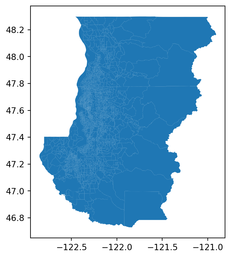

Geospatial Operations

Geopandas can carry out all standard GIS operations using methods implemented on a GeoDataFrame, for example

• clip: “cut” the extent of one dataset using the boundaries of another
• dissolve: aggregate geometries using a common value from an attribute (e.g. remove interior boundaries from larger container polygons, e.g. counties within a state)
• simplify: remove vertices from the input geometries
• buffer: extend the boundaries of input geometries by a fixed distance (always returns polygons)
• centroid: compute the geometric center of input geometries (always returns points)
• convex/concave hull: compute the most efficient convex/convave polygon that contains vertices from all input geometries

By combining these operations along with spatial predicates, we can create queries based on the topological relationships between two sets of geographic units, which is often critical for creating variables of interest.

To demonstrate, we will first collect data from OpenStreetMap (OSM), specifically highways in the Seattle metro. In OSM parlance, this means we’re querying for “highways” with the “motorway” tag (which means “the highest-performance roads within a territory. It should be used only on roads with control of access, or selected roads with limited access depending on the local context and prevailing convention. Those roads are generally referred to as motorways, freeways or expressways in English.”)

import osmnx as ox

highways = ox.features_from_polygon(
    sea_ejscreen.union_all(), tags={"highway": "motorway"}
)

This returns a new GeoDataFrame storing each highway as a line feature.

highways.head()

		geometry	highway	ref	fixme	payment:good_to_go	source	name	lit	bus:lanes	hgv	...	motorcycle:lanes:conditional	sidewalk	hov:lanes:backward	hov:lanes:forward	hazmat	start_date	sidewalk:left	sidewalk:right	bridge:movable	wikidata
element	id
way	4634293	LINESTRING (-122.31862 47.64265, -122.3177 47....	motorway	WA 520	NaN	NaN	NaN	NaN	NaN	NaN	NaN	...	NaN	NaN	NaN	NaN	NaN	NaN	NaN	NaN	NaN	NaN
	4644156	LINESTRING (-122.32264 47.65701, -122.3226 47....	motorway	I 5	NaN	NaN	NaN	Ship Canal Bridge	yes	NaN	designated	...	NaN	NaN	NaN	NaN	NaN	NaN	NaN	NaN	NaN	NaN
	4644167	LINESTRING (-122.32242 47.6467, -122.3224 47.6...	motorway	I 5	NaN	NaN	NaN	Ship Canal Bridge	yes	NaN	designated	...	NaN	NaN	NaN	NaN	NaN	NaN	NaN	NaN	NaN	NaN
	4644173	LINESTRING (-122.32265 47.6467, -122.32258 47....	motorway	I 5 Express	NaN	NaN	NaN	Ship Canal Bridge	yes	NaN	NaN	...	NaN	NaN	NaN	NaN	NaN	NaN	NaN	NaN	NaN	NaN
	4709507	LINESTRING (-122.32598 47.73592, -122.32558 47...	motorway	I 5	NaN	NaN	NaN	NaN	NaN	designated|||	designated	...	NaN	NaN	NaN	NaN	NaN	NaN	NaN	NaN	NaN	NaN

5 rows × 104 columns

highways.plot()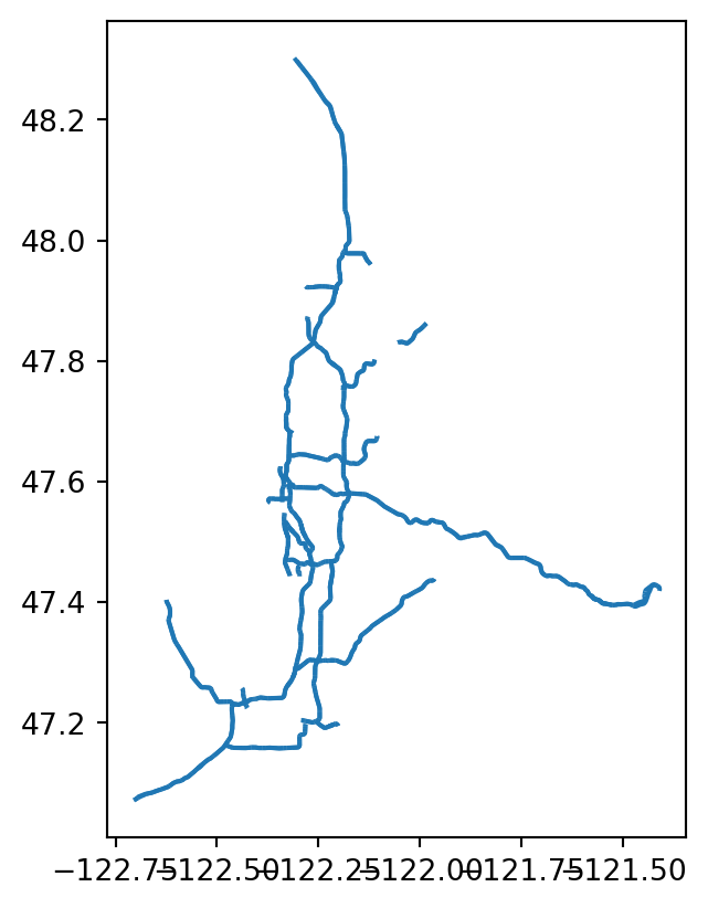

Notice in the call to features_from_polygon above, we used the unary_union operator on the Seattle tracts dataframe. This effectively combines all the tracts into a single polygon so we are querying anything that intersects any tract, rather than querying intersections with each tract individually. We can do the same thing on the highway GeoDataFrame to see the effect

# note in geopandas <1.0 this is `highways.unary_union`

hw_union = highways.union_all()

hw_union

Now hw_union is a single shapely.Polygon with no attribute information

gpd.GeoDataFrame(geometry=[hw_union], crs=4326).explore(tiles='CartoDB Positron')

Make this Notebook Trusted to load map: File -> Trust Notebook

Integrating Spatial Datasets

Let’s assume the role of a public health epidemiologist who is interested in equity issues surrounding exposure to highways and automobile emissions. We may be interested in who lives near the highway and whether the population nearby experiences a heightened exposure to toxic emissions.

Select by Location

One simple question would be, which tracts have a highway run through them? We can formalize that by asking which tracts intersect the highway system.

highway_blockgroups = sea_ejscreen[sea_ejscreen.intersects(hw_union)]
highway_blockgroups.plot()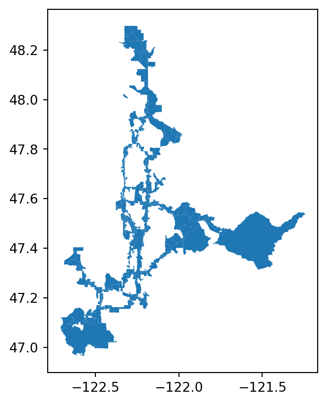

A more complicated question is, which tracts are within 1.5km of a road? This is ‘complicated’ because it forces us to formalize an ill-defined relationship: the distance between a polygon and the nearest point on a line. What does it mean for the polygon to be ‘within’ 1.5km? Does that mean the whole tract? most of it? any part of it?

If we can define a most suitable distance measure, the technical selection is easy to execute using an intermediate geometry.

road_buffer = highways.to_crs(highways.estimate_utm_crs()).buffer(1500)

gpd.GeoDataFrame(geometry=[road_buffer.union_all()], crs=road_buffer.crs).explore(tiles='CartoDB Positron')

Make this Notebook Trusted to load map: File -> Trust Notebook

sea_ejscreen.crs

<Geographic 2D CRS: EPSG:4326>
Name: WGS 84
Axis Info [ellipsoidal]:
- Lat[north]: Geodetic latitude (degree)
- Lon[east]: Geodetic longitude (degree)
Area of Use:
- name: World.
- bounds: (-180.0, -90.0, 180.0, 90.0)
Datum: World Geodetic System 1984 ensemble
- Ellipsoid: WGS 84
- Prime Meridian: Greenwich

sea_ejscreen[sea_ejscreen.intersects(road_buffer.union_all())]

	geoid	ACSTOTPOP	ACSIPOVBAS	ACSEDUCBAS	ACSTOTHH	ACSTOTHU	MINORPOP	MINORPCT	LOWINCOME	LOWINCPCT	...	T_PM25_P2	T_PM25_P6	AREALAND	AREAWATER	NPL_CNT	TSDF_CNT	Shape_Length	Shape_Area	geometry	year

0 rows × 368 columns

This gives us back nothing… There is no intersection because the EJSCREEN data is still stored in Lat/Long, but we reprojected the road buffer into UTM

sea_ejscreen = sea_ejscreen.to_crs(road_buffer.crs)

By selecting the tracts that intersect with the interstate buffer, we are codifying the tracts as ‘near the highway’ if any portion of a tract is within 1.5km. This can be an awkard choice when polygons are irregularly shaped or heteogeneously sized (Census tracts are both). This means large tracts get included as ‘near’, even when a small portion of the polygon is within the 1.5km threshold (like the tract on the far Eastern edge).

sea_ejscreen[sea_ejscreen.intersects(road_buffer.union_all())].plot()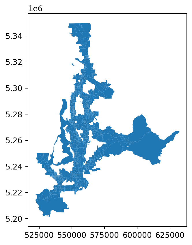

Alternatively, we might ask, which tracts have their center within 1.5km of a highway? Or more formally, which tracts have their centroids intersect with the 1500m buffer.

sea_ejscreen[sea_ejscreen.centroid.intersects(road_buffer.union_all())].plot()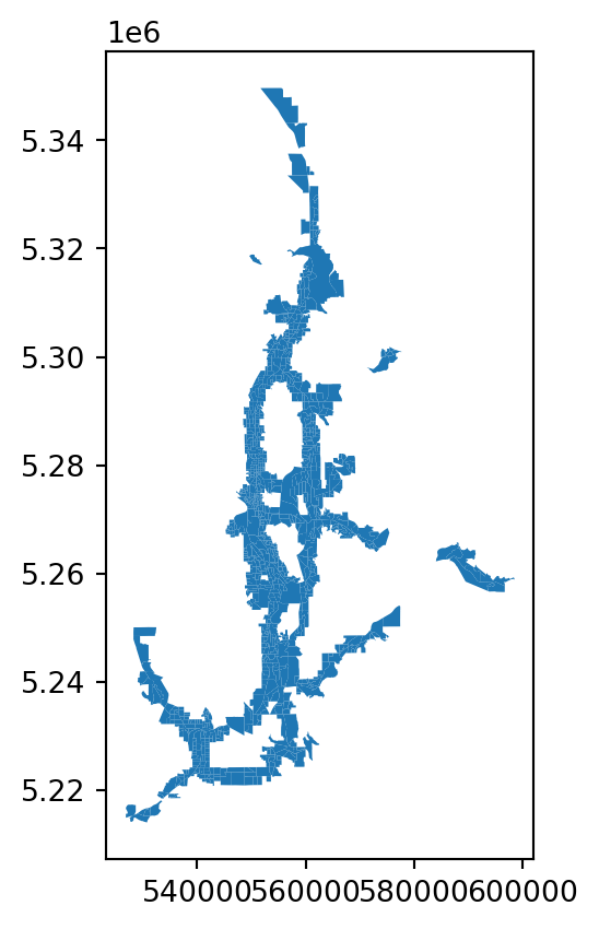

If we are happy with that definition of proximity, we can use the spatial selection to create and update a new attribute on the dataframe. Here, we will select the tracts whose centroids are within the threshold distance, then create a new column called “highway_buffer”, set to “inside” (using the indices of the spatial selection to define which rows are being set).

# get the dataframe index of the tracts intersecting the buffer

inside_idx = sea_ejscreen[
    sea_ejscreen.centroid.intersects(road_buffer.union_all())
].index

# set the 'highway_buffer' attribute to 'inside' for the indices within
sea_ejscreen.loc[inside_idx, "highway_buffer"] = "inside"

# fill all NaN values in the column with 'outside'
sea_ejscreen["highway_buffer"] = sea_ejscreen["highway_buffer"].fillna("outside").astype('category')

Now ‘highway_buffer’ is a binary variable defining whether a tract is “near” a highway or not. We could have set these values to one and zero, but setting them as a categorical variable means that the geopandas plot method uses a different kind of coloring scheme that matches the data more appropriately.

sea_ejscreen[['highway_buffer', 'geometry']].explore("highway_buffer", legend=True, tiles='CartoDB Positron')

Make this Notebook Trusted to load map: File -> Trust Notebook

Then, we can use this spatial distinction as a grouping variable to look at average values inside versus outside the threshold zone.

sea_ejscreen.groupby("highway_buffer")[["PM25", "DSLPM", "MINORPCT"]].mean()

/tmp/ipykernel_17288/860608503.py:1: FutureWarning: The default of observed=False is deprecated and will be changed to True in a future version of pandas. Pass observed=False to retain current behavior or observed=True to adopt the future default and silence this warning.
  sea_ejscreen.groupby("highway_buffer")[["PM25", "DSLPM", "MINORPCT"]].mean()

	PM25	DSLPM	MINORPCT
highway_buffer
inside	6.298818	1.043487	0.404843
outside	6.061902	0.723160	0.283832

On average, both PM2.5 and Disel Particulate Matter levels are higher for tracts located within 1.5km of an OSM ‘motorway’ (what we think is probably an interstate highway). The share of residents identifying as a racial or ethnic miority is also 12% higher on average.

Spatial Join

In the example above, we use only the geometric relationship between observations to make selections from one dataset. In other cases, we need to attach attribute data from one dataset to the other using spatial relationships. For example we might want to count the number of health clinics that fall inside each census tract. This actually entails two operations: attaching census tract identifiers to each clinic, then aggregating by tract identifier and counting all clinics within

Once again we will query OSM, this time looking for an amenity with the ‘clinic’ tag

clinics = ox.features_from_polygon(
    sea_ejscreen.to_crs(4326).union_all(), tags={"amenity": "clinic"}
)
clinics = clinics.reset_index().set_index("id")

clinics.head()

	element	geometry	amenity	healthcare	name	brand	brand:wikidata	healthcare:counselling	operator	operator:wikidata	...	start_date	ele	gnis:feature_id	ref	building:material	waste_disposal	wikidata	owner	layer	type
id
1242268219	node	POINT (-122.11025 47.67027)	clinic	clinic	Overlake Clinics - Urgent Care	NaN	NaN	NaN	NaN	NaN	...	NaN	NaN	NaN	NaN	NaN	NaN	NaN	NaN	NaN	NaN
1248759443	node	POINT (-122.35027 47.64978)	clinic	clinic	ZoomCare	ZoomCare	Q64120374	NaN	ZoomCare	Q64120374	...	NaN	NaN	NaN	NaN	NaN	NaN	NaN	NaN	NaN	NaN
1273816342	node	POINT (-122.18631 47.62807)	clinic	clinic	Evergreen Integrative Medicine L.L.P.	NaN	NaN	NaN	NaN	NaN	...	NaN	NaN	NaN	NaN	NaN	NaN	NaN	NaN	NaN	NaN
1273816350	node	POINT (-122.186 47.62807)	clinic	clinic	Romanick MD PLLC	NaN	NaN	NaN	NaN	NaN	...	NaN	NaN	NaN	NaN	NaN	NaN	NaN	NaN	NaN	NaN
1381933749	node	POINT (-122.18496 47.62548)	clinic	clinic	Medical Arts Associates	NaN	NaN	NaN	NaN	NaN	...	NaN	NaN	NaN	NaN	NaN	NaN	NaN	NaN	NaN	NaN

5 rows × 110 columns

The clinics dataset now has manuy types of clinics, and also has a mixed geometry type; some clinics are stored as polygons (where the building footprint has been digitized) whereas others are simply stored as points. Lets filter the dataset to include only those defined as clinic (e.g. not counseling) and only points (not polygons)

We can do this in two steps like

clinics = clinics[(clinics.healthcare == "clinic") & (clinics.element == "node")]

clinics.explore(tiles='CartoDB Positron', tooltip=['name', 'healthcare'])

Make this Notebook Trusted to load map: File -> Trust Notebook

clinics = clinics.to_crs(sea_ejscreen.crs)

clinics_geoid = clinics.sjoin(sea_ejscreen[["geoid", "geometry"]])

clinics_geoid.head()

	element	geometry	amenity	healthcare	name	brand	brand:wikidata	healthcare:counselling	operator	operator:wikidata	...	gnis:feature_id	ref	building:material	waste_disposal	wikidata	owner	layer	type	index_right	geoid
id
1242268219	node	POINT (566792.704 5280036.188)	clinic	clinic	Overlake Clinics - Urgent Care	NaN	NaN	NaN	NaN	NaN	...	NaN	NaN	NaN	NaN	NaN	NaN	NaN	NaN	1326	530330323092
1248759443	node	POINT (548794.035 5277580.42)	clinic	clinic	ZoomCare	ZoomCare	Q64120374	NaN	ZoomCare	Q64120374	...	NaN	NaN	NaN	NaN	NaN	NaN	NaN	NaN	172	530330049002
1273816342	node	POINT (561132.643 5275283.673)	clinic	clinic	Evergreen Integrative Medicine L.L.P.	NaN	NaN	NaN	NaN	NaN	...	NaN	NaN	NaN	NaN	NaN	NaN	NaN	NaN	699	530330237003
1273816350	node	POINT (561155.932 5275284.017)	clinic	clinic	Romanick MD PLLC	NaN	NaN	NaN	NaN	NaN	...	NaN	NaN	NaN	NaN	NaN	NaN	NaN	NaN	699	530330237003
1381933749	node	POINT (561236.936 5274997.501)	clinic	clinic	Medical Arts Associates	NaN	NaN	NaN	NaN	NaN	...	NaN	NaN	NaN	NaN	NaN	NaN	NaN	NaN	699	530330237003

5 rows × 112 columns

Now we want to count clinics in each geoid. Since we know osmid uniquely identifies each clinic, we can reset the index, then groupby the ‘geoid’ variable, counting the unique ’osmid’s in each one

clinic_count = clinics_geoid.reset_index().groupby("geoid").count()["id"]

clinic_count

geoid
530330001003    1
530330002002    1
530330006004    2
530330012004    1
530330013003    1
               ..
530610519252    1
530610527072    1
530610535093    1
530610538023    1
530610538024    1
Name: id, Length: 177, dtype: int64

clinic_count is now a pandas series where the index refers to the census tract of interest and the value corresponds to the number of clinics that fall inside.

sea_ejscreen = sea_ejscreen.merge(
    clinic_count.rename("clinic_count"), left_on="geoid", right_index=True, how="left"
)

sea_ejscreen.clinic_count

0       NaN
1       NaN
2       1.0
3       NaN
4       NaN
       ... 
2478    NaN
2479    NaN
2480    NaN
2481    NaN
2482    NaN
Name: clinic_count, Length: 2483, dtype: float64

Now the sea_ejscreen GeoDataFrame has a new column called ‘clinic_count’ that holds the number of clinics inside. Since we know that NaN (Not a number) refers to zero in this case, we can go ahead and fill the missing data.

sea_ejscreen["clinic_count"] = sea_ejscreen["clinic_count"].fillna(0)

sea_ejscreen[['clinic_count', 'geometry']].explore(
    "clinic_count", scheme='fisher_jenks', cmap='Reds', tiles='CartoDB DarkMatter', style_kwds=dict(weight=0.2)
)

Make this Notebook Trusted to load map: File -> Trust Notebook