Centrography refers to a set of descriptive statistics that provide summary descriptions of point patterns.
This notebook introduces three types of centrography analysis for point patterns in pysal.
Central Tendency
Dispersion and Orientation
Shape Analysis
We also illustrate centrography analysis using two simulated datasets. See Another Example
Central Tendency
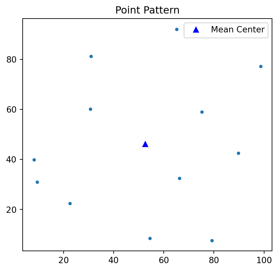
mean_center: calculate the mean center of the unmarked point pattern.
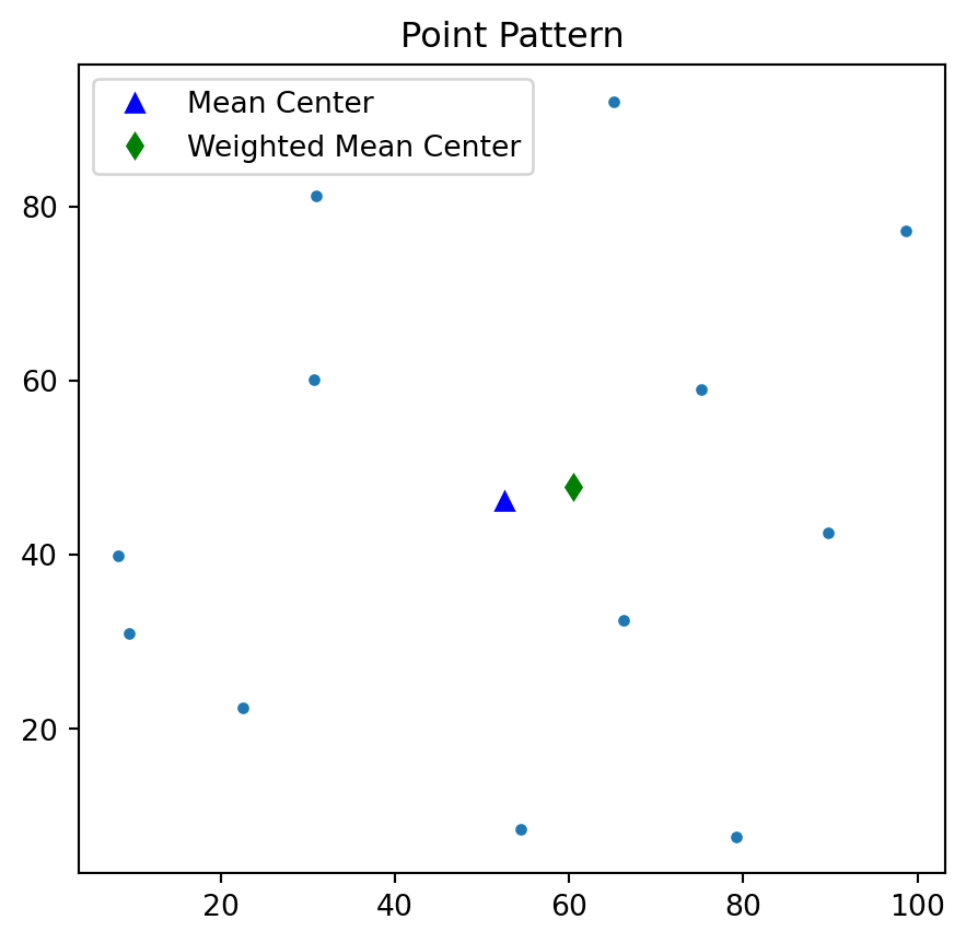
weighted_mean_center: calculate the weighted mean center of the marked point pattern.
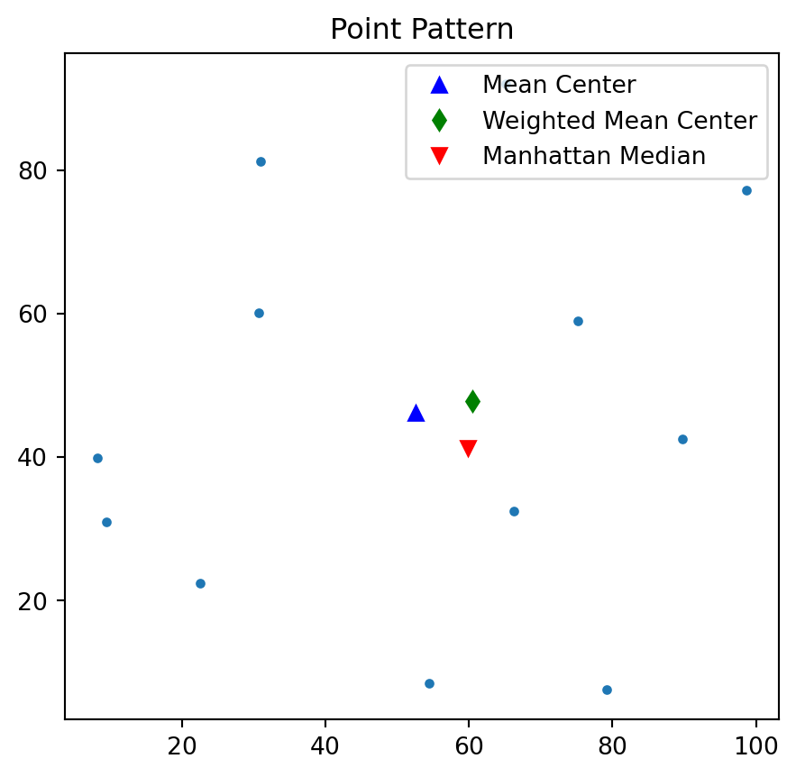
manhattan_median: calculate the manhattan median
euclidean_median: calculate the Euclidean median
Dispersion and Orientation
std_distance: calculate the standard distance
standard deviational ellipse
Shape Analysis
hull: calculate the convex hull of the point pattern
mbr: calculate the minimum bounding box (rectangle)
All of the above functions operate on a series of coordinate pairs. That is, the data type of the first argument should be \((n,2)\) array_like. In case that you have a point pattern (PointPattern instance), you need to pass its attribute “points” instead of itself to these functions.
import numpy as npfrom pointpats import PointPattern%matplotlib inlineimport matplotlib.pyplot as pltpoints = [[66.22, 32.54], [22.52, 22.39], [31.01, 81.21], [9.47, 31.02], [30.78, 60.10], [75.21, 58.93], [79.26, 7.68], [8.23, 39.93], [98.73, 77.17], [89.78, 42.53], [65.19, 92.08], [54.46, 8.48]]pp = PointPattern(points) #create a point pattern "pp" from listpp.points
x
y
0
66.22
32.54
1
22.52
22.39
2
31.01
81.21
3
9.47
31.02
4
30.78
60.10
5
75.21
58.93
6
79.26
7.68
7
8.23
39.93
8
98.73
77.17
9
89.78
42.53
10
65.19
92.08
11
54.46
8.48
type(pp.points)
pandas.core.frame.DataFrame
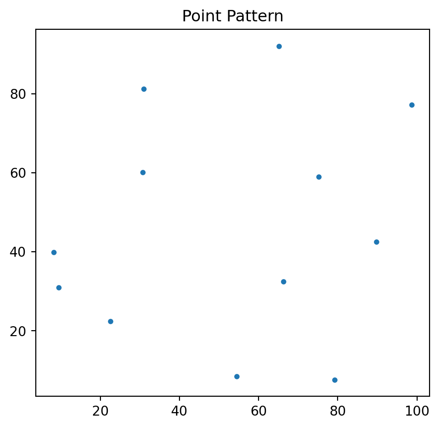
We can use PointPattern class method plot to visualize pp.
pp.plot()
from pointpats.centrography import (hull, mbr, mean_center,
                                    weighted_mean_center, manhattan_median,
                                    std_distance,euclidean_median,ellipse)
Central Tendency
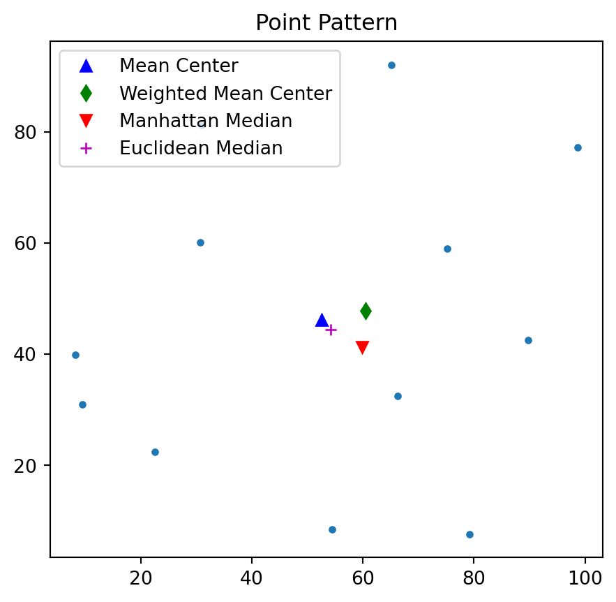
Central Tendency concerns about the center point of the two-dimensional distribution. It is similar to the first moment of a one-dimensional distribution. There are several ways to measure central tendency, each having pros and cons. We need to carefully select the appropriate measure according to our objective and data status.
The Weighted mean center is meant for marked point patterns. Aside from the first argument which is a series of \((x,y)\) coordinates in weighted_mean_center function, we need to specify its second argument which is the weight for each event point.
weights = np.arange(12)weights
array([ 0, 1, 2, 3, 4, 5, 6, 7, 8, 9, 10, 11])
wmc = weighted_mean_center(pp.points, weights)wmc
array([60.51681818, 47.76848485])
pp.plot() #use class method "plot" to visualize point patternplt.plot(mc[0], mc[1], 'b^', label='Mean Center') plt.plot(wmc[0], wmc[1], 'gd', label='Weighted Mean Center')plt.legend(numpoints=1)
The Manhattan median is the location which minimizes the absolute distance to all the event points. It is an extension of the median measure in one-dimensional space to two-dimensional space. Since in one-dimensional space, a median is the number separating the higher half of a dataset from the lower half, we define the Manhattan median as a tuple whose first element is the median of \(x\) coordinates and second element is the median of \(y\) coordinates.
Though Manhattan median can be found very quickly, it is not unique if you have even number of points. In this case, pysal handles the Manhattan median the same way as numpy.median: return the average of the two middle values.
#get the number of points in point pattern "pp"pp.n
12
#Manhattan Median is not unique for "pp"mm = manhattan_median(pp.points)mm
/home/serge/miniforge3/envs/workshop-pysal/lib/python3.10/site-packages/pointpats/centrography.py:216: UserWarning: Manhattan Median is not unique for even point patterns.
  warnings.warn(s)
The Euclidean Median is the location from which the sum of the Euclidean distances to all points in a distribution is a minimum. It is an optimization problem and very important for more general location allocation problems. There is no closed form solution. We can use first iterative algorithm (Kuhn and Kuenne, 1962) to approximate Euclidean Median.
Below, we define a function named median_center with the first argument points a series of \((x,y)\) coordinates and the second argument crit the convergence criterion.
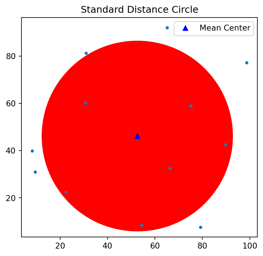
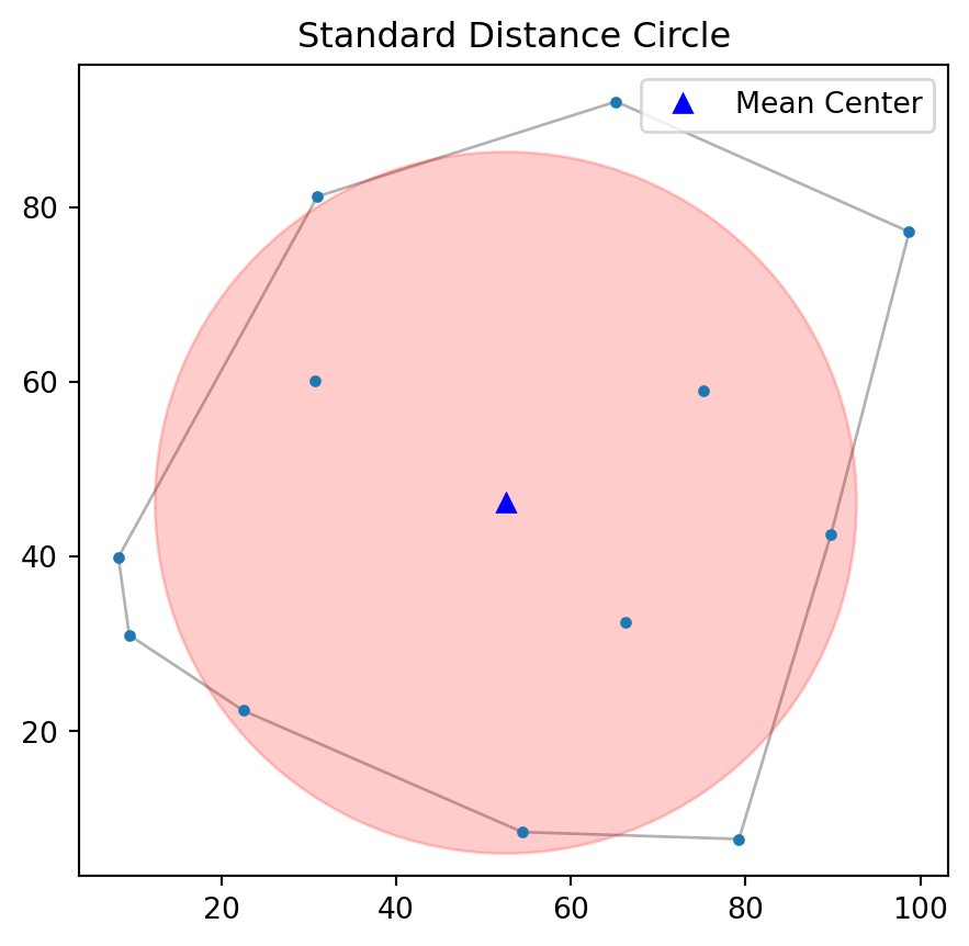
The Standard distance is closely related to the usual definition of the standard deviation of a data set, and it provides a measure of how dispersed the events are around their mean center \((x_m,y_m)\). Taken together, these measurements can be used to plot a summary circle (standard distance circle) for the point pattern, centered at \((x_m,y_m)\) with radius \(SD\), as shown below.
stdd = std_distance(pp.points)stdd
np.float64(40.14980648908671)
Plot mean center as well as the standard distance circle.
From the above figure, we can observe that there are five points outside the standard distance circle which are potential outliers.
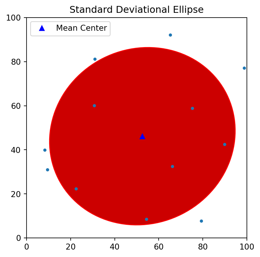
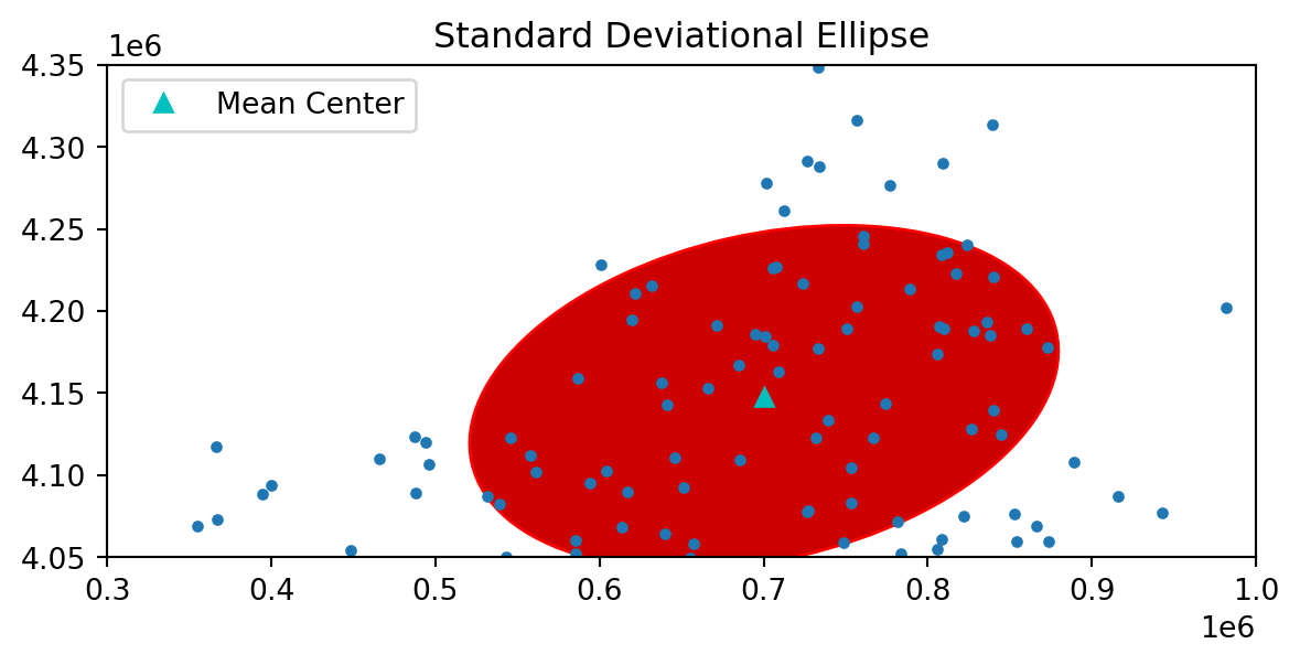
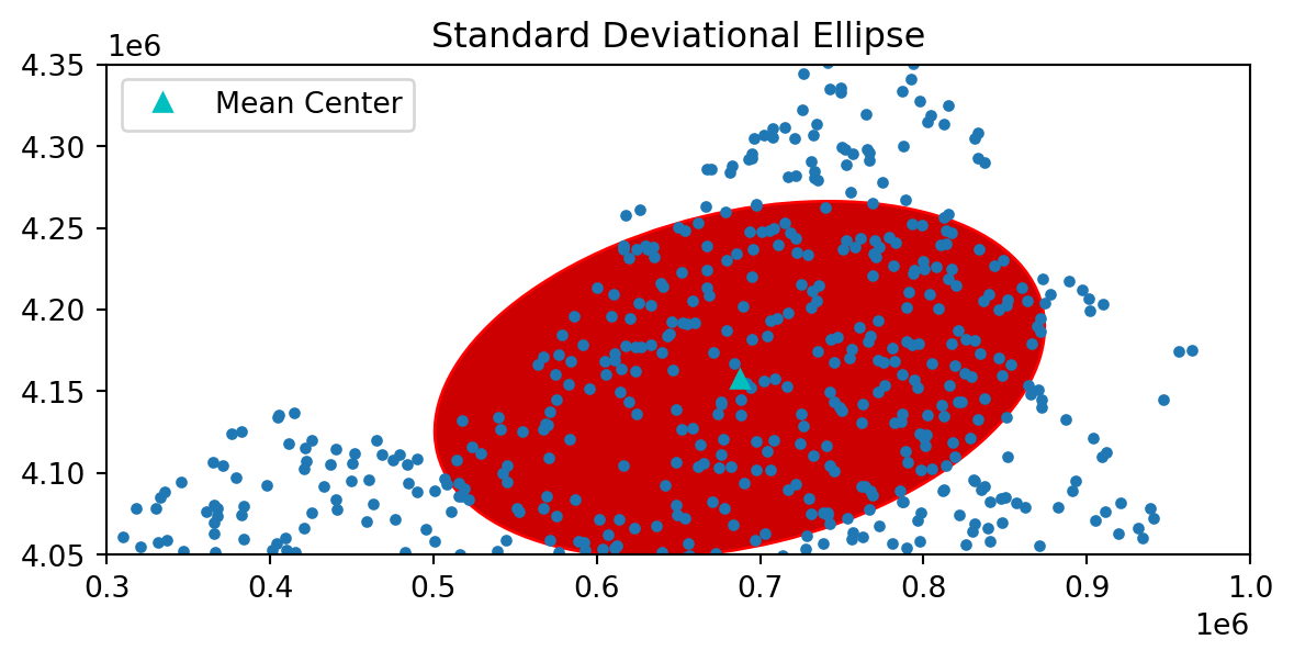
Standard Deviational Ellipse
Compared with standard distance circle which measures dispersion using a single parameter \(SD\), standard deviational ellipse measures dispersion and trend in two dimensions through angle of rotation \(\theta\), dispersion along major axis \(s_x\) and dispersion along minor axis \(s_y\):
Major axis defines the direction of maximum spread in the distribution. \(s_x\) is the semi-major axis (half the length of the major axis):
Minor axis defines the direction of minimum spread and is orthogonal to major axis. \(s_y\) is the semi-minor axis (half the length of the minor axis):
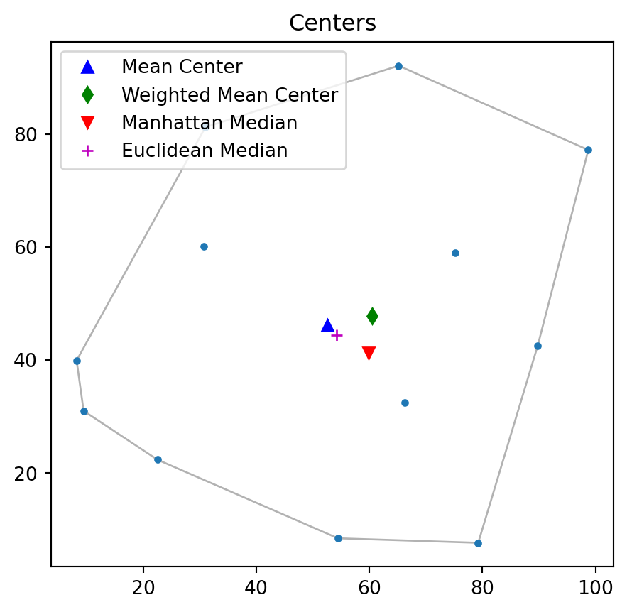
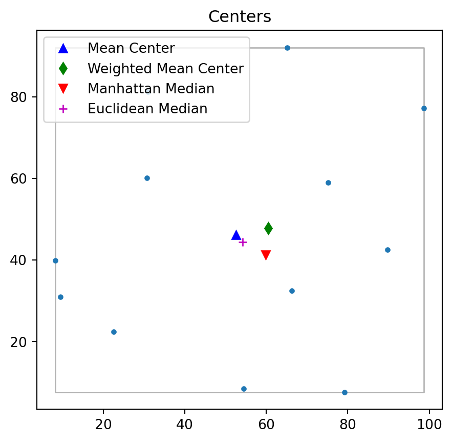
By specifying “hull” argument True in PointPattern class method plot, we can easily plot convex hull of the point pattern.
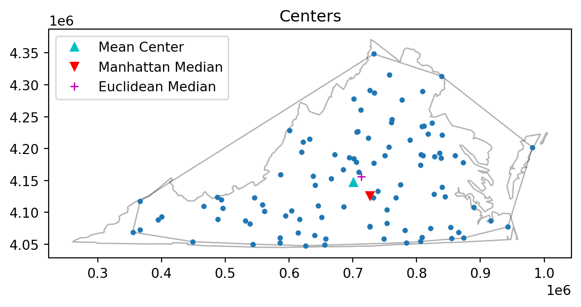
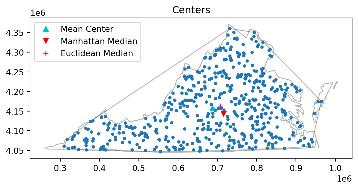
pp.plot(title='Centers', hull=True ) #plot point pattern "pp" as well as its convex hullplt.plot(mc[0], mc[1], 'b^', label='Mean Center')plt.plot(wmc[0], wmc[1], 'gd', label='Weighted Mean Center')plt.plot(mm[0], mm[1], 'rv', label='Manhattan Median')plt.plot(em[0], em[1], 'm+', label='Euclidean Median')plt.legend(numpoints=1)
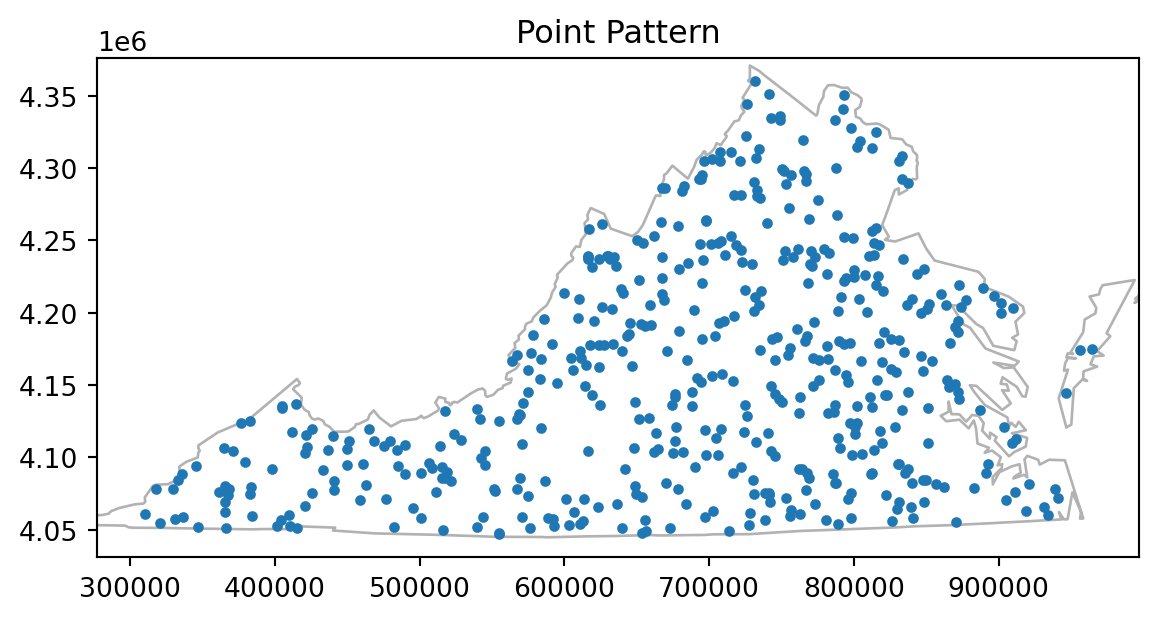
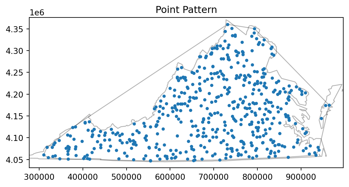
We apply the centrography statistics and visualization to 2 simulated random datasets.
#from pysal.contrib import shapely_extfrom libpysal.cg import shapely_extfrom pointpats import PoissonPointProcess as csrimport libpysal as psfrom pointpats import as_window#import pysal_examples# open "vautm17n" polygon shapefileva = ps.io.open(ps.examples.get_path("vautm17n.shp"))# Create the exterior polygons for VA from the union of the county shapespolys = [shp for shp in va]state = shapely_ext.cascaded_union(polys)
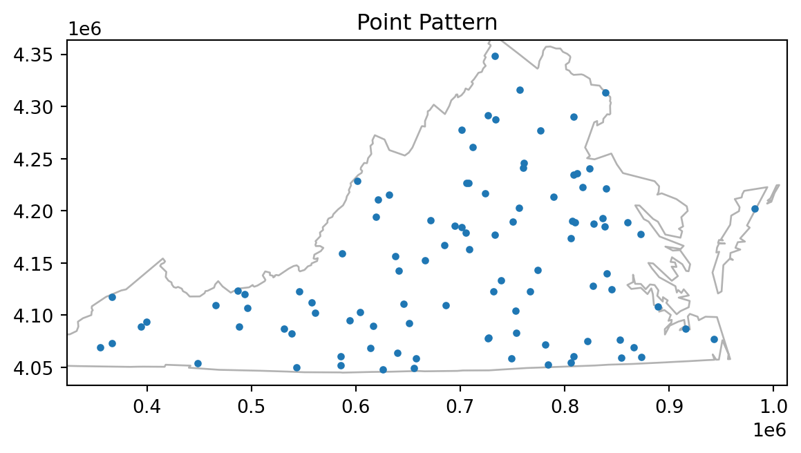
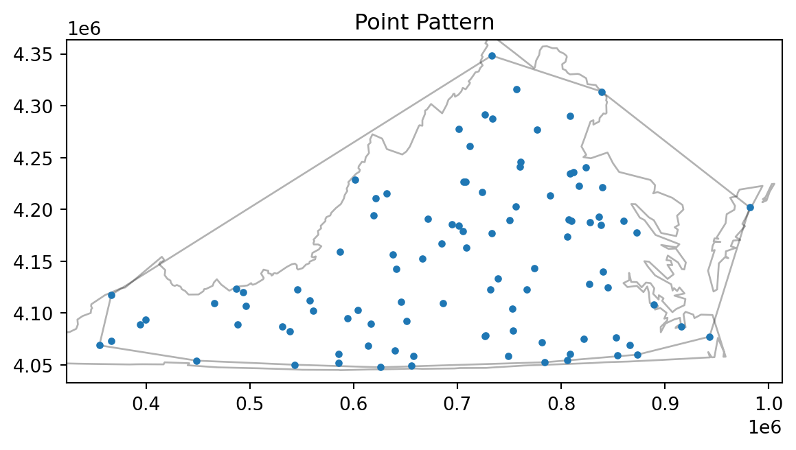
Simulate a 100-point dataset within VA state border from a CSR (complete spatial randomness) process.
If we calculate the Euclidean distances between every event point and Mean Center (Euclidean Median), and sum them up, we can see that Euclidean Median is the optimal point in iterms of minimizing the Euclidean distances to all the event points.
from pointpats import dtotprint(dtot(mc, pp.points))print(dtot(em, pp.points))print(dtot(mc, pp.points) > dtot(em, pp.points))
72394703.08771706
71935834.58259372
True
Source Code
---title: Centrography for Point Patternsauthor: "Serge Rey"jupyter: python3format: html: theme: light: flatly dark: darkly toc: true code-fold: false---## Introduction*Centrography* refers to a set of descriptive statistics that provide summary descriptions of point patterns.This notebook introduces three types of centrography analysis for point patterns in pysal.* Central Tendency* Dispersion and Orientation* Shape AnalysisWe also illustrate centrography analysis using two simulated datasets. See [Another Example](#Another-Example)* Central Tendency 1. mean_center: calculate the mean center of the unmarked point pattern. 2. weighted_mean_center: calculate the weighted mean center of the marked point pattern. 3. manhattan_median: calculate the manhattan median 4. euclidean_median: calculate the Euclidean median* Dispersion and Orientation 1. std_distance: calculate the standard distance 2. standard deviational ellipse* Shape Analysis 1. hull: calculate the convex hull of the point pattern 2. mbr: calculate the minimum bounding box (rectangle)All of the above functions operate on a series of coordinate pairs. That is, the data type of the first argument should be $(n,2)$ array_like. In case that you have a point pattern (PointPattern instance), you need to pass its attribute "points" instead of itself to these functions.```{python}#| warning: falseimport numpy as npfrom pointpats import PointPattern%matplotlib inlineimport matplotlib.pyplot as pltpoints = [[66.22, 32.54], [22.52, 22.39], [31.01, 81.21], [9.47, 31.02], [30.78, 60.10], [75.21, 58.93], [79.26, 7.68], [8.23, 39.93], [98.73, 77.17], [89.78, 42.53], [65.19, 92.08], [54.46, 8.48]]pp = PointPattern(points) #create a point pattern "pp" from listpp.points ``````{python}#| warning: falsetype(pp.points)```We can use PointPattern class method **plot** to visualize **pp**.```{python}pp.plot()``````{python}from pointpats.centrography import (hull, mbr, mean_center, weighted_mean_center, manhattan_median, std_distance,euclidean_median,ellipse)```# Central TendencyCentral Tendency concerns about the center point of the two-dimensional distribution. It is similar to the first moment of a one-dimensional distribution. There are several ways to measure central tendency, each having pros and cons. We need to carefully select the appropriate measure according to our objective and data status.## Mean Center $(x_{mc},y_{mc})$$$x_{mc}=\frac{1}{n} \sum^n_{i=1}x_i$$$$y_{mc}=\frac{1}{n} \sum^n_{i=1}y_i$$```{python}mc = mean_center(pp.points)mc``````{python}pp.plot()plt.plot(mc[0], mc[1], 'b^', label='Mean Center')plt.legend(numpoints=1)```## Weighted Mean Center $(x_{wmc},y_{wmc})$$$x_{wmc}=\sum^n_{i=1} \frac{w_i x_i}{\sum^n_{i=1}w_i}$$$$y_{wmc}=\sum^n_{i=1} \frac{w_i y_i}{\sum^n_{i=1}w_i}$$The Weighted mean center is meant for marked point patterns. Aside from the first argument which is a series of $(x,y)$ coordinates in **weighted_mean_center** function, we need to specify its second argument which is the weight for each event point.```{python}weights = np.arange(12)weights``````{python}wmc = weighted_mean_center(pp.points, weights)wmc``````{python}pp.plot() #use class method "plot" to visualize point patternplt.plot(mc[0], mc[1], 'b^', label='Mean Center') plt.plot(wmc[0], wmc[1], 'gd', label='Weighted Mean Center')plt.legend(numpoints=1)```## Manhattan Median $(x_{mm},y_{mm})$$$min f(x_{mm},y_{mm})= \sum^n_{i=1}(|x_i-x_{mm}|+|y_i-y_{mm}|)$$The Manhattan median is the location which minimizes the absolute distance to all the event points. It is an extension of the median measure in one-dimensional space to two-dimensional space. Since in one-dimensional space, a median is the number separating the higher half of a dataset from the lower half, we define the Manhattan median as a tuple whose first element is the median of $x$ coordinates and second element is the median of $y$ coordinates.Though Manhattan median can be found very quickly, it is not unique if you have even number of points. In this case, pysal handles the Manhattan median the same way as numpy.median: return the average of the two middle values.```{python}#get the number of points in point pattern "pp"pp.n``````{python}#Manhattan Median is not unique for "pp"mm = manhattan_median(pp.points)mm``````{python}pp.plot()plt.plot(mc[0], mc[1], 'b^', label='Mean Center')plt.plot(wmc[0], wmc[1], 'gd', label='Weighted Mean Center')plt.plot(mm[0], mm[1], 'rv', label='Manhattan Median')plt.legend(numpoints=1)```## Euclidean Median $(x_{em},y_{em})$$$min f(x_{em},y_{em})= \sum^n_{i=1} \sqrt{(x_i-x_{em})^2+(y_i-y_{em})^2}$$The Euclidean Median is the location from which the sum of the Euclidean distances to all points in a distribution is a minimum. It is an optimization problem and very important for more general location allocation problems. There is no closed form solution. We can use first iterative algorithm (Kuhn and Kuenne, 1962) to approximate Euclidean Median. Below, we define a function named median_center with the first argument **points** a series of $(x,y)$ coordinates and the second argument **crit** the convergence criterion.```{python}def median_center(points, crit=0.0001): points = np.asarray(points) x0, y0 = points.mean(axis=0) dx = np.inf dy = np.inf iteration =0while np.abs(dx) > crit or np.abs(dy) > crit: xd = points[:, 0] - x0 yd = points[:, 1] - y0 d = np.sqrt(xd*xd + yd*yd) w =1./d w = w / w.sum() x1 = w * points[:, 0] x1 = x1.sum() y1 = w * points[:, 1] y1 = y1.sum() dx = x1 - x0 dy = y1 - y0 iteration +=1print(x0, x1, dx, dy, d.sum(), iteration) x0 = x1 y0 = y1return x1, y1``````{python}median_center(pp.points, crit=.0001)```After 18 iterations, the convergence criterion is reached. The Euclidean Median is $(54.167594287646125,44.424308658832047)$.We can also call the function **euclidean_median** in pysal to calculate the Euclidean Median.```{python}em = euclidean_median(pp.points)em```The two results we get from **euclidean_median** function in pysal and the **median_center** function we define here are very much the same.```{python}pp.plot()plt.plot(mc[0], mc[1], 'b^', label='Mean Center')plt.plot(wmc[0], wmc[1], 'gd', label='Weighted Mean Center')plt.plot(mm[0], mm[1], 'rv', label='Manhattan Median')plt.plot(em[0], em[1], 'm+', label='Euclidean Median')plt.legend(numpoints=1)```# Dispersion and Orientation## Standard Distance & Standard Distance Circle$$SD = \displaystyle \sqrt{\frac{\sum^n_{i=1}(x_i-x_{m})^2}{n} + \frac{\sum^n_{i=1}(y_i-y_{m})^2}{n}}$$The Standard distance is closely related to the usual definition of the standard deviation of a data set, and it provides a measure of how dispersed the events are around their mean center $(x_m,y_m)$. Taken together, these measurements can be used to plot a summary circle (standard distance circle) for the point pattern, centered at $(x_m,y_m)$ with radius $SD$, as shown below.```{python}stdd = std_distance(pp.points)stdd```Plot mean center as well as the standard distance circle.```{python}circle1=plt.Circle((mc[0], mc[1]),stdd,color='r')ax = pp.plot(get_ax=True, title='Standard Distance Circle')ax.add_artist(circle1)plt.plot(mc[0], mc[1], 'b^', label='Mean Center')ax.set_aspect('equal')plt.legend(numpoints=1)```From the above figure, we can observe that there are five points outside the standard distance circle which are potential outliers.## Standard Deviational EllipseCompared with standard distance circle which measures dispersion using a single parameter $SD$, standard deviational ellipse measures dispersion and trend in two dimensions through angle of rotation $\theta$, dispersion along major axis $s_x$ and dispersion along minor axis $s_y$:* Major axis defines the direction of maximum spread in the distribution. $s_x$ is the semi-major axis (half the length of the major axis):$$ s_x = \displaystyle \sqrt{\frac{2(\sum_{i=1}^n (x_i-\bar{x})\cos(\theta) - \sum_{i=1}^n (y_i-\bar{y})\sin(\theta))^2}{n-2}}$$* Minor axis defines the direction of minimum spread and is orthogonal to major axis. $s_y$ is the semi-minor axis (half the length of the minor axis):$$ s_y = \displaystyle \sqrt{\frac{2(\sum_{i=1}^n (x_i-\bar{x})\sin(\theta) - \sum_{i=1}^n (y_i-\bar{y})\cos(\theta))^2}{n-2}}$$* The ellipse is rotated clockwise through an angle $\theta$:$$\theta = \displaystyle \arctan{\{ (\sum_i(x_i-\bar{x})^2-\sum_i(y_i-\bar{y})^2) + \frac{[(\sum_i(x_i-\bar{x})^2-\sum_i(y_i-\bar{y})^2)^2 + 4(\sum_i(x-\bar{x})(y_i-\bar{y}))^2]^\frac{1}{2}}{2\sum_i(x-\bar{x})(y_i-\bar{y})}\}}$$```{python}sx, sy, theta = ellipse(pp.points)sx, sy, theta``````{python}theta_degree = np.degrees(theta) #need degree of rotation to plot the ellipsetheta_degree```The Standard Deviational Ellipse for the point pattern is rotated clockwise by $63.25^{\circ}$.```{python}from matplotlib.patches import Ellipsefrom pylab import figure, show,randfig = figure()#ax = fig.add_subplot(111, aspect='equal')e = Ellipse(xy=mean_center(pp.points), width=sx*2, height=sy*2, angle=-theta_degree) #angle is rotation in degrees (anti-clockwise)ax = pp.plot(get_ax=True, title='Standard Deviational Ellipse')ax.add_artist(e)e.set_clip_box(ax.bbox)e.set_facecolor([0.8,0,0])e.set_edgecolor([1,0,0])ax.set_xlim(0,100)ax.set_ylim(0,100)ax.set_aspect('equal')plt.plot(mc[0], mc[1], 'b^', label='Mean Center')plt.legend(numpoints=1)show()```# Shape Analysis## [Convex Hull](https://en.wikipedia.org/wiki/Convex_hull)The convex hull of a point pattern *pp* is the smallest convex set that contains *pp*. We can call function **hull** to caculate the convex hull.```{python}hull(pp.points)```By specifying "hull" argument **True** in PointPattern class method **plot**, we can easily plot convex hull of the point pattern.```{python}pp.plot(title='Centers', hull=True ) #plot point pattern "pp" as well as its convex hullplt.plot(mc[0], mc[1], 'b^', label='Mean Center')plt.plot(wmc[0], wmc[1], 'gd', label='Weighted Mean Center')plt.plot(mm[0], mm[1], 'rv', label='Manhattan Median')plt.plot(em[0], em[1], 'm+', label='Euclidean Median')plt.legend(numpoints=1)```## [Minimum Bounding Rectangle](https://en.wikipedia.org/wiki/Minimum_bounding_rectangle)Minimum Bounding Rectangle (Box) is the same as the minimum bounding Rectangle of its convex hull. Thus, it is almost always bigger than convex hull.We can call **mbr** function to calculate the leftmost, downmost, rightmost, and upmost value of the vertices of minimum bounding rectangle.```{python}mbr(pp.points)```Thus, four vertices of the minimum bounding rectangle is $(8.23,7.68),(98.73,7.68),(98.73,92.08),(8.23,92.08)$.```{python}pp.plot(title='Centers', window=True ) #plot point pattern "pp" as well as its Minimum Bounding Rectangleplt.plot(mc[0], mc[1], 'b^', label='Mean Center')plt.plot(wmc[0], wmc[1], 'gd', label='Weighted Mean Center')plt.plot(mm[0], mm[1], 'rv', label='Manhattan Median')plt.plot(em[0], em[1], 'm+', label='Euclidean Median')plt.legend(numpoints=1)``````{python}pp.plot(title='Centers', hull=True , window=True )#plot point pattern "pp", convex hull, and Minimum Bounding Rectangleplt.plot(mc[0], mc[1], 'b^', label='Mean Center')plt.plot(wmc[0], wmc[1], 'gd', label='Weighted Mean Center')plt.plot(mm[0], mm[1], 'rv', label='Manhattan Median')plt.plot(em[0], em[1], 'm+', label='Euclidean Median')plt.legend(numpoints=1)```Plot Standard Distance Circle and Convex Hull.```{python}circle1=plt.Circle((mc[0], mc[1]),stdd,color='r',alpha=0.2)ax = pp.plot(get_ax=True, title='Standard Distance Circle', hull=True)ax.add_artist(circle1)plt.plot(mc[0], mc[1], 'b^', label='Mean Center')ax.set_aspect('equal')plt.legend(numpoints=1)```# Another ExampleWe apply the centrography statistics and visualization to 2 simulated random datasets.```{python}#| warning: false#from pysal.contrib import shapely_extfrom libpysal.cg import shapely_extfrom pointpats import PoissonPointProcess as csrimport libpysal as psfrom pointpats import as_window#import pysal_examples# open "vautm17n" polygon shapefileva = ps.io.open(ps.examples.get_path("vautm17n.shp"))# Create the exterior polygons for VA from the union of the county shapespolys = [shp for shp in va]state = shapely_ext.cascaded_union(polys)```## Simulate a 100-point dataset within VA state border from a CSR (complete spatial randomness) process.```{python}#| warning: falsepp = csr(as_window(state), 100, 1, asPP=True).realizations[0]pp.plot(window=True)``````{python}#| warning: falsepp.plot(window=True, hull=True)``````{python}#| warning: falsemc = mean_center(pp.points)mm = manhattan_median(pp.points)em = euclidean_median(pp.points)pp.plot(title='Centers', hull=True , window=True )#plot point pattern "pp", convex hull, and Minimum Bounding Rectangleplt.plot(mc[0], mc[1], 'c^', label='Mean Center')plt.plot(mm[0], mm[1], 'rv', label='Manhattan Median')plt.plot(em[0], em[1], 'm+', label='Euclidean Median')plt.legend(numpoints=1)```Plot Standard Distance Circle of the simulated point pattern.```{python}#| warning: falsesx, sy, theta = ellipse(pp.points)sx, sy, thetatheta_degree = np.degrees(theta) #need degree of rotation to plot the ellipsefrom matplotlib.patches import Ellipsefrom pylab import figure, show,randfig = figure()#ax = fig.add_subplot(111, aspect='equal')e = Ellipse(xy=mean_center(pp.points), width=sx*2, height=sy*2, angle=-theta_degree)ax = pp.plot(get_ax=True, title='Standard Deviational Ellipse')ax.add_artist(e)e.set_clip_box(ax.bbox)e.set_facecolor([0.8,0,0])e.set_edgecolor([1,0,0])ax.set_xlim(300000,1000000)ax.set_ylim(4050000,4350000)#ax.set_aspect('equal')plt.plot(mc[0], mc[1], 'c^', label='Mean Center')plt.legend(numpoints=1)show()```## Simulate a 500-point dataset within VA state border from a CSR (complete spatial randomness) process.```{python}#| warning: falsepp = csr(as_window(state), 500, 1, asPP=True).realizations[0]pp.plot(window=True)``````{python}#| warning: falsepp.plot(window=True, hull=True)``````{python}#| warning: falsemc = mean_center(pp.points)mm = manhattan_median(pp.points)em = euclidean_median(pp.points)pp.plot(title='Centers', hull=True , window=True )#plot point pattern "pp", convex hull, and Minimum Bounding Rectangleplt.plot(mc[0], mc[1], 'c^', label='Mean Center')plt.plot(mm[0], mm[1], 'rv', label='Manhattan Median')plt.plot(em[0], em[1], 'm+', label='Euclidean Median')plt.legend(numpoints=1)``````{python}#| warning: falsesx, sy, theta = ellipse(pp.points)sx, sy, thetatheta_degree = np.degrees(theta) #need degree of rotation to plot the ellipsefrom matplotlib.patches import Ellipsefrom pylab import figure, show,randfig = figure()#ax = fig.add_subplot(111, aspect='equal')e = Ellipse(xy=mean_center(pp.points), width=sx*2, height=sy*2, angle=-theta_degree)ax = pp.plot(get_ax=True, title='Standard Deviational Ellipse')ax.add_artist(e)e.set_clip_box(ax.bbox)e.set_facecolor([0.8,0,0])e.set_edgecolor([1,0,0])ax.set_xlim(300000,1000000)ax.set_ylim(4050000,4350000)#ax.set_aspect('equal')plt.plot(mc[0], mc[1], 'c^', label='Mean Center')plt.legend(numpoints=1)show()```If we calculate the Euclidean distances between every event point and Mean Center (Euclidean Median), and sum them up, we can see that Euclidean Median is the optimal point in iterms of minimizing the Euclidean distances to all the event points.```{python}#| warning: falsefrom pointpats import dtotprint(dtot(mc, pp.points))print(dtot(em, pp.points))print(dtot(mc, pp.points) > dtot(em, pp.points))```