Visualization for Area Unit Data
Plotting the Geometries

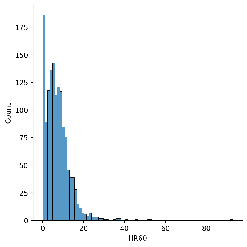
Plotting the attribute distribution
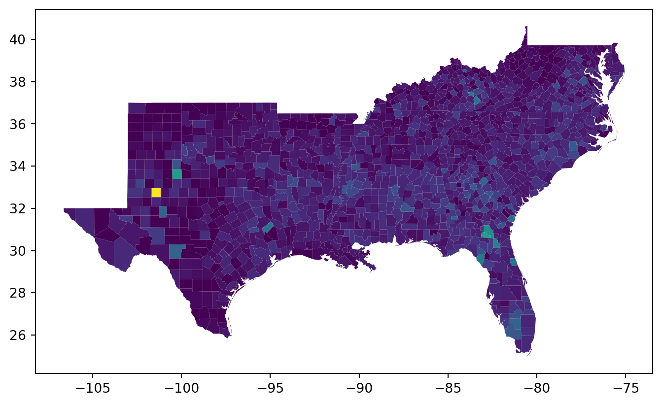
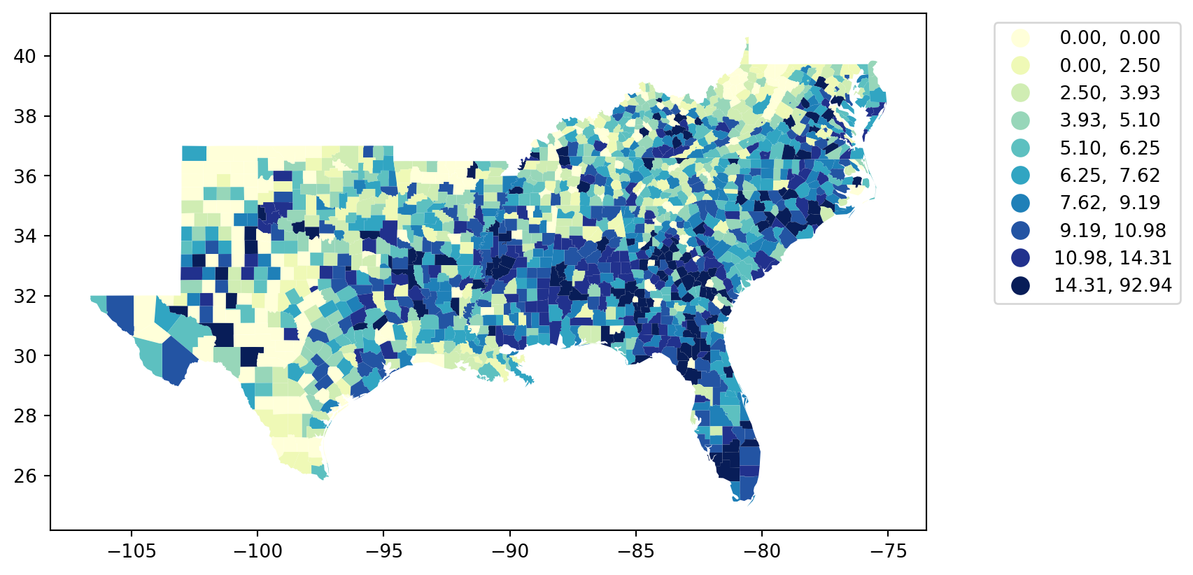
Spatial Distribution (Default Choropleth)
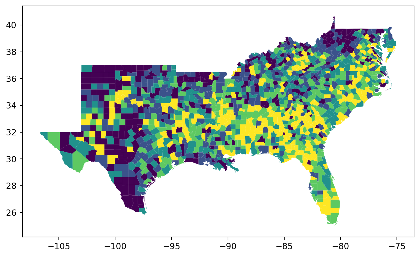
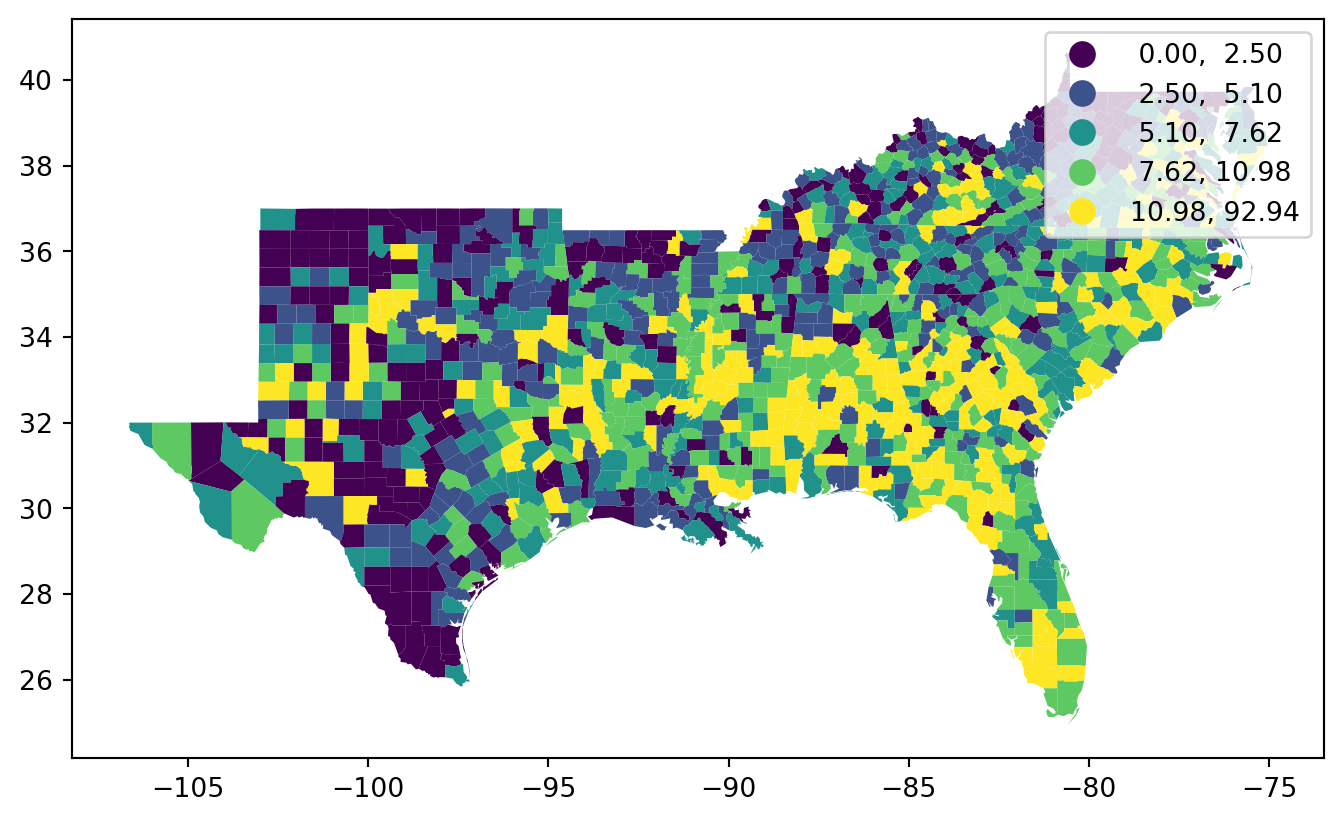
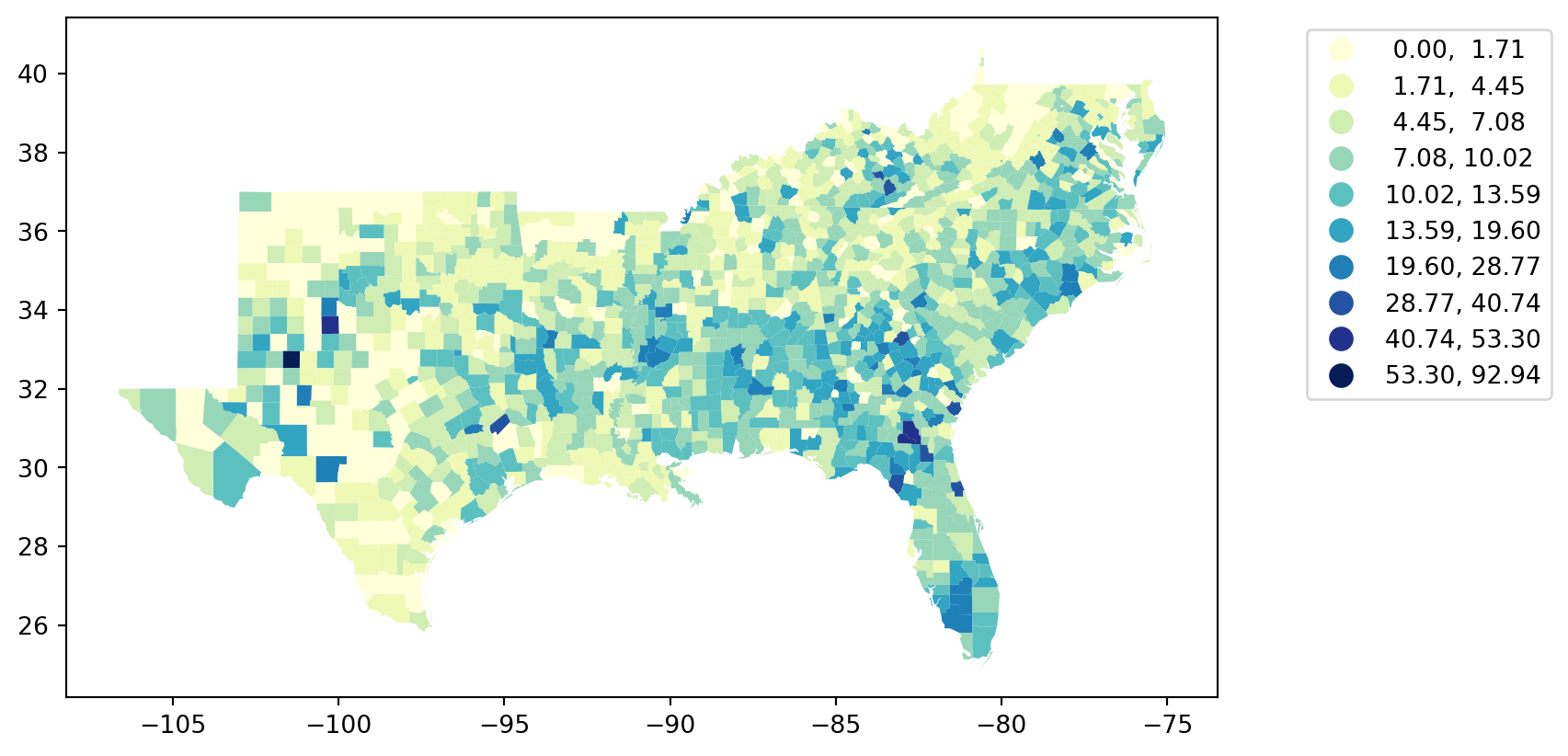
Spatial Distribution (Changing the classification)
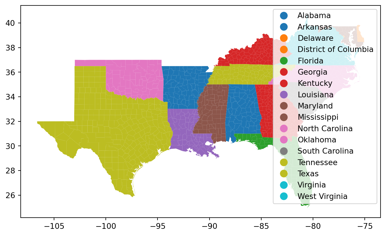
Spatial Distribution (Adding a legend)
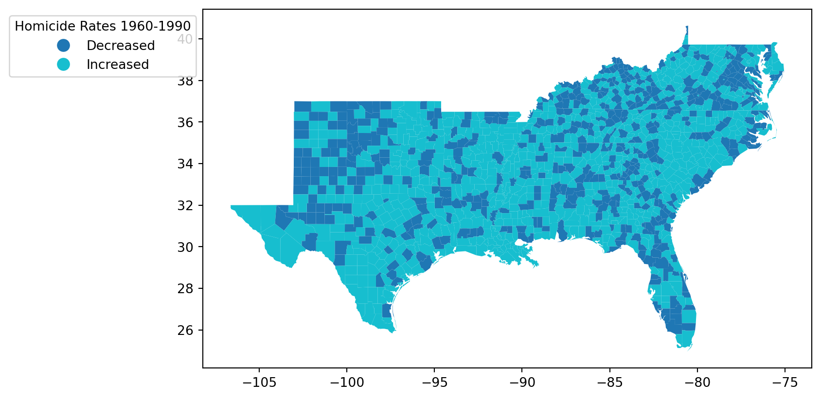
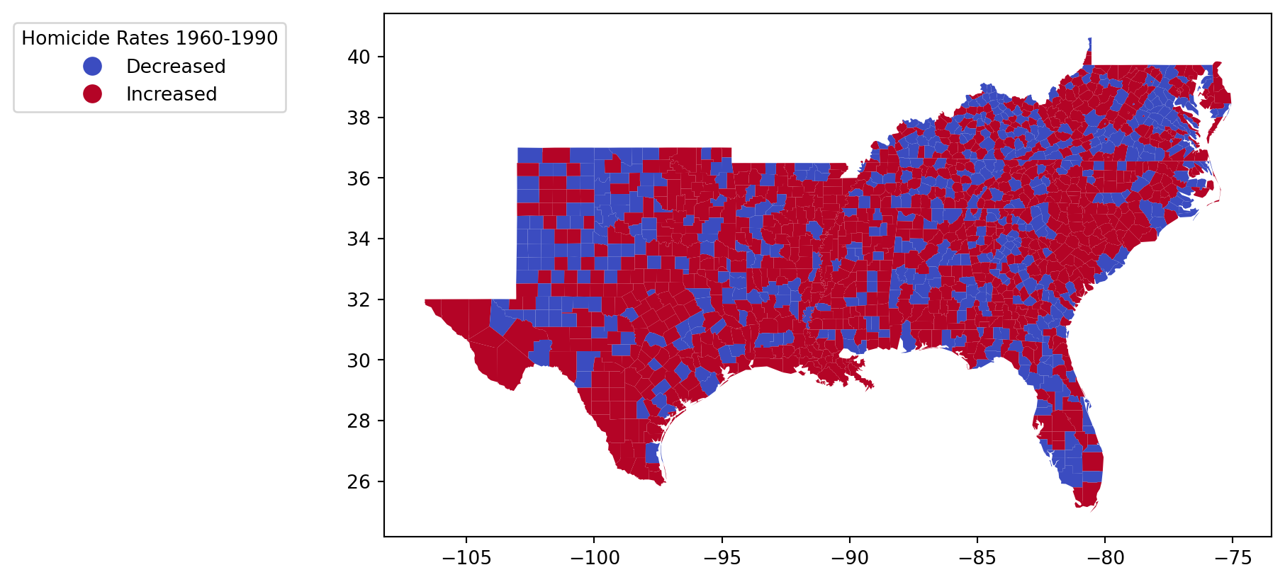
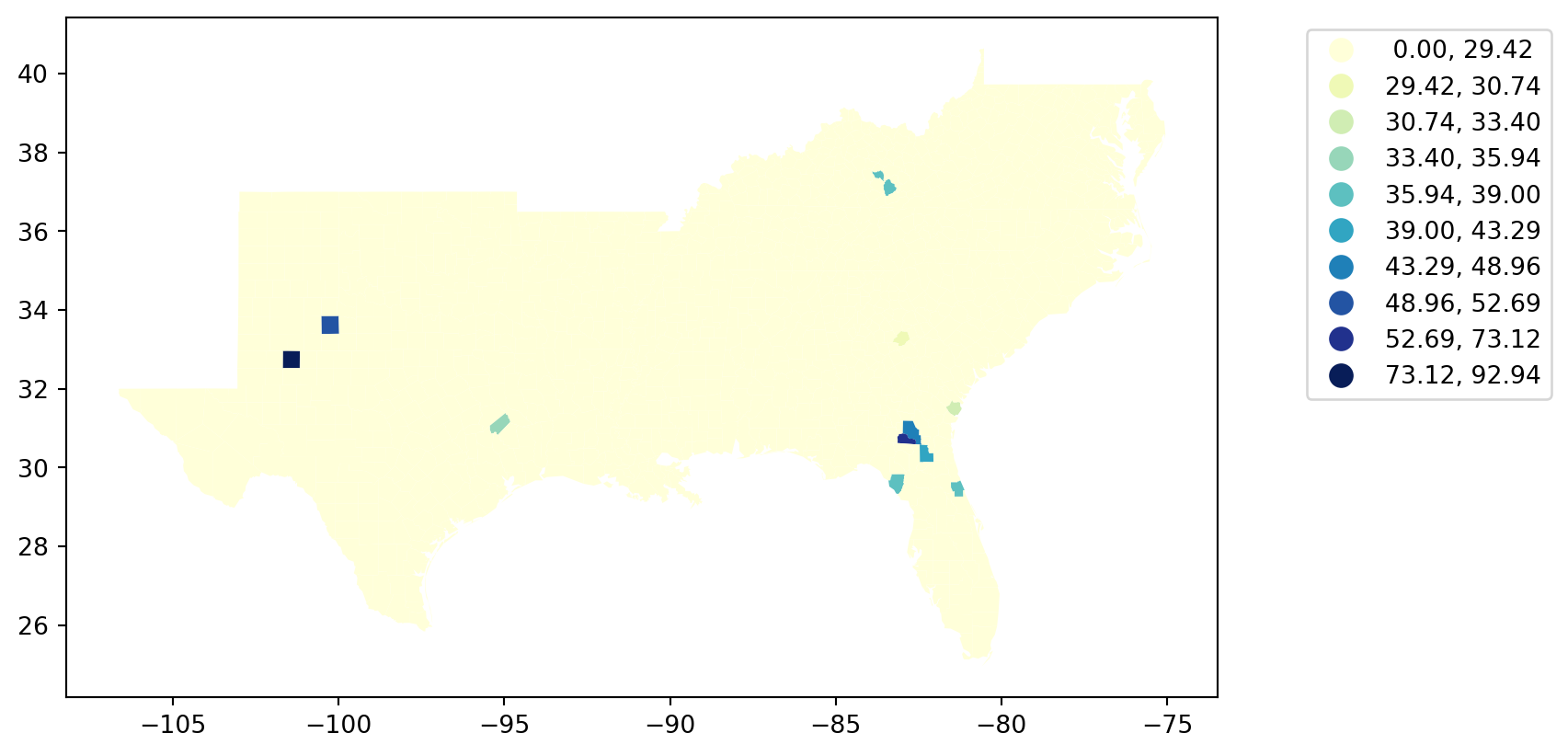
Mapping the Boolean variable
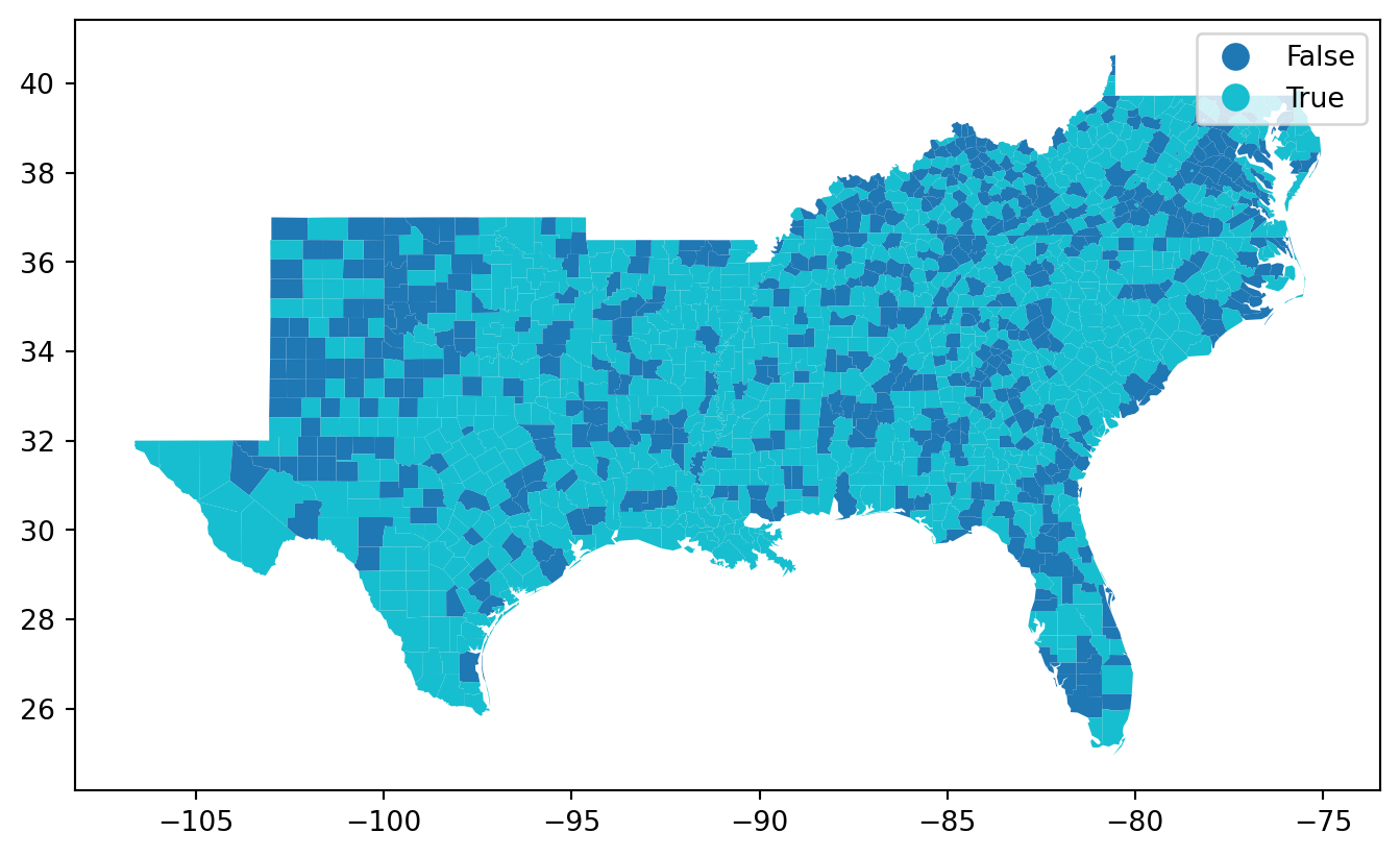
Map the new variable

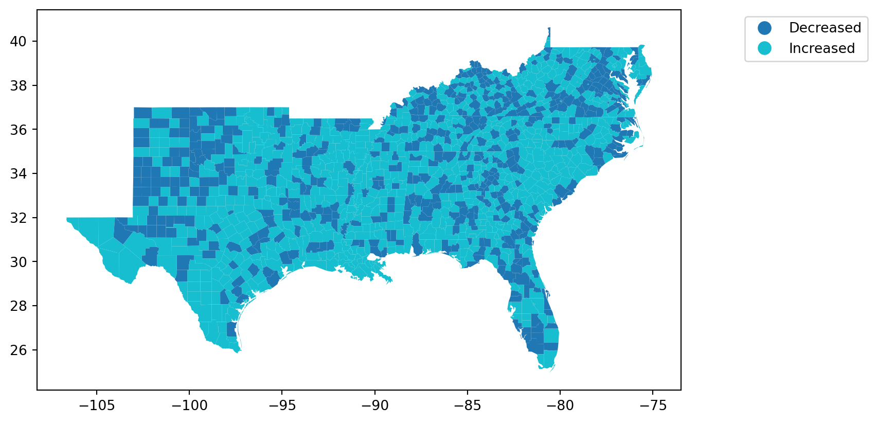
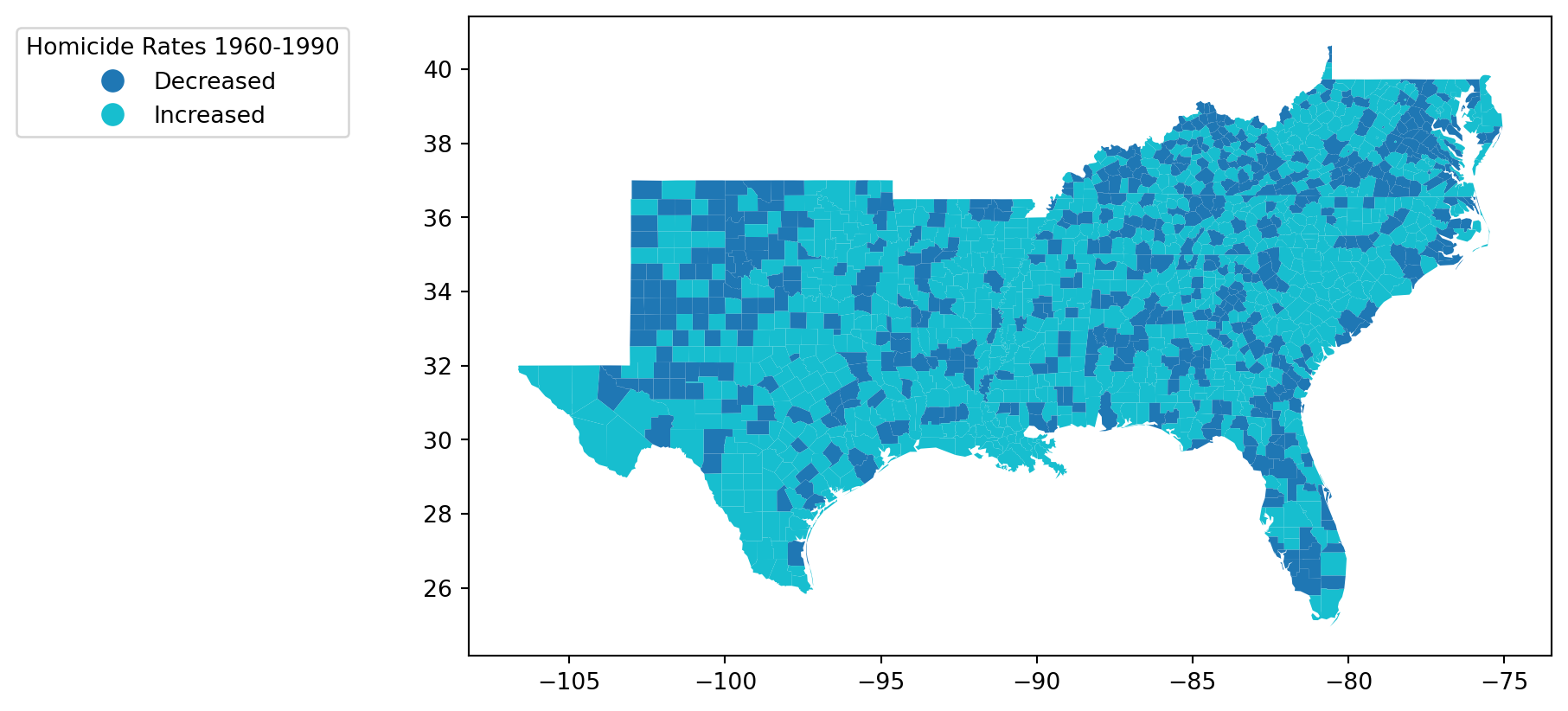
Legend Positioning
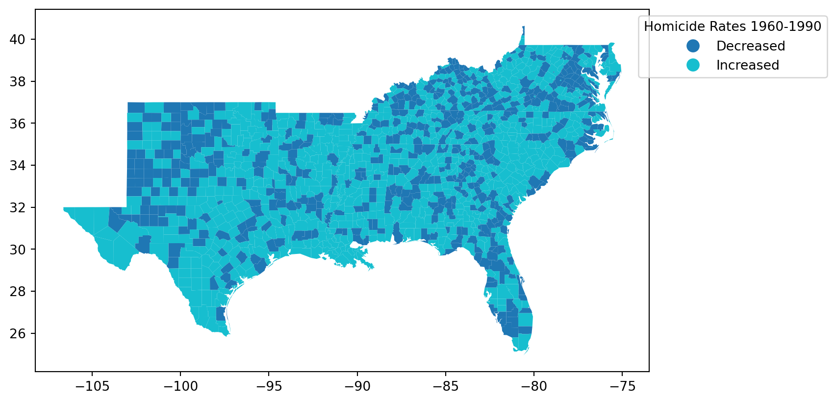
Legend Title
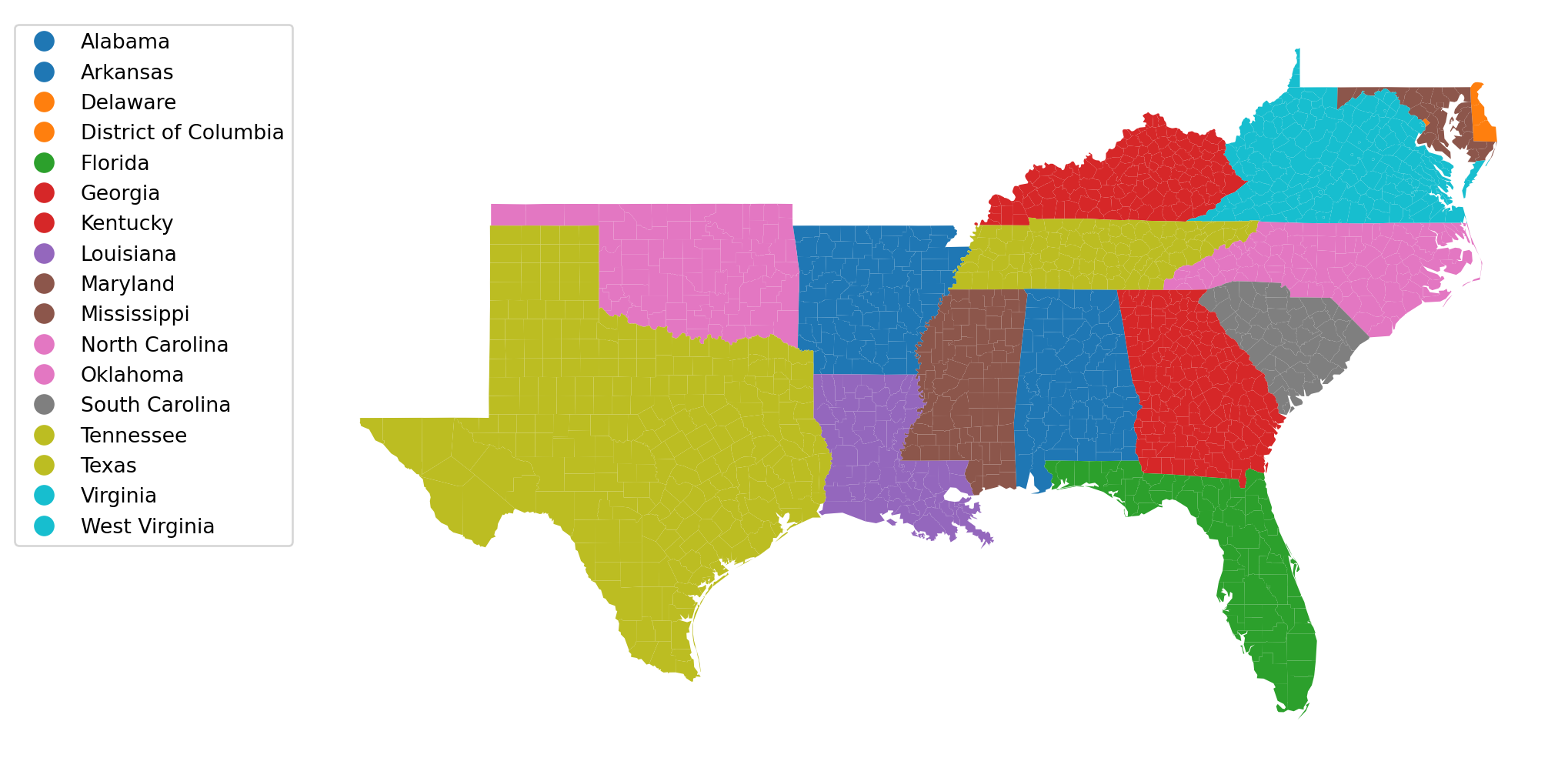
More Adjustments
More Adjustments
Color schemes
- matplotlib (hunter2007Matplotlib2Da?)
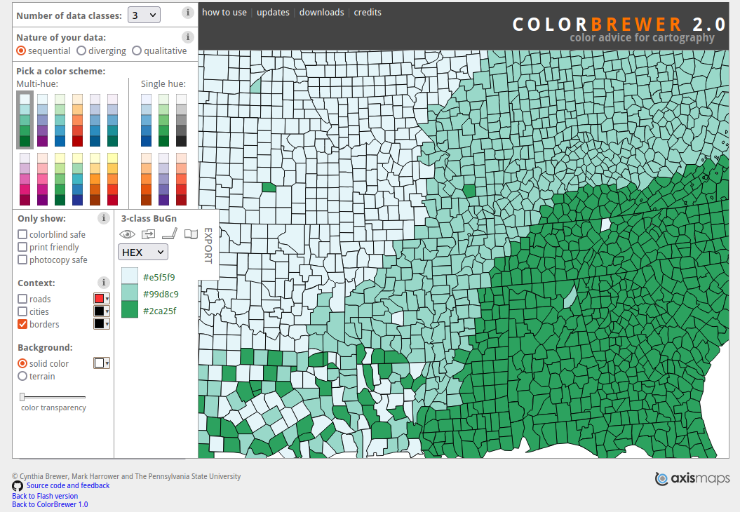
- ColorBrewer Harrower and Brewer (2003)
![colorbrewer]()
Sequential Color Schemes
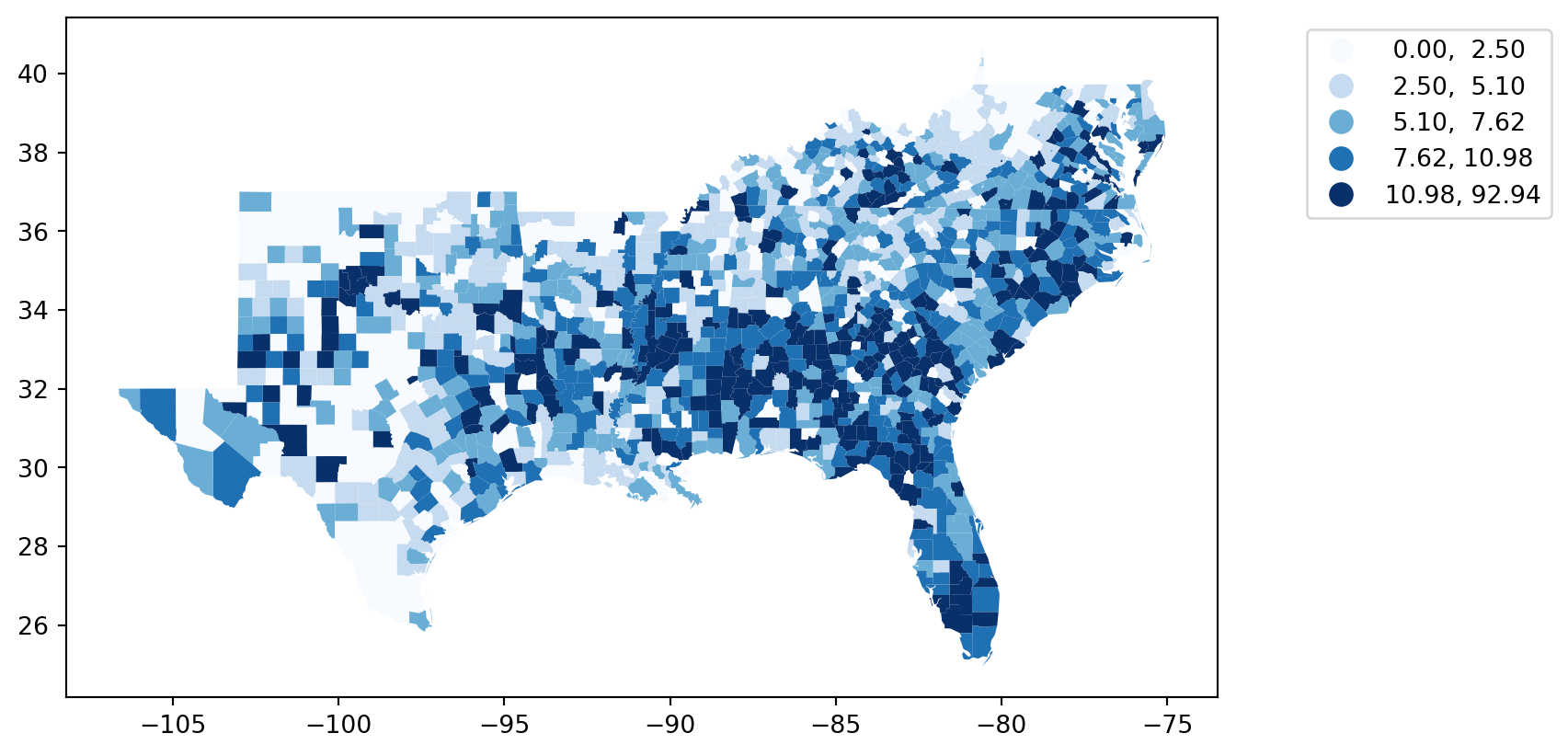
Change the color map: Single Hue
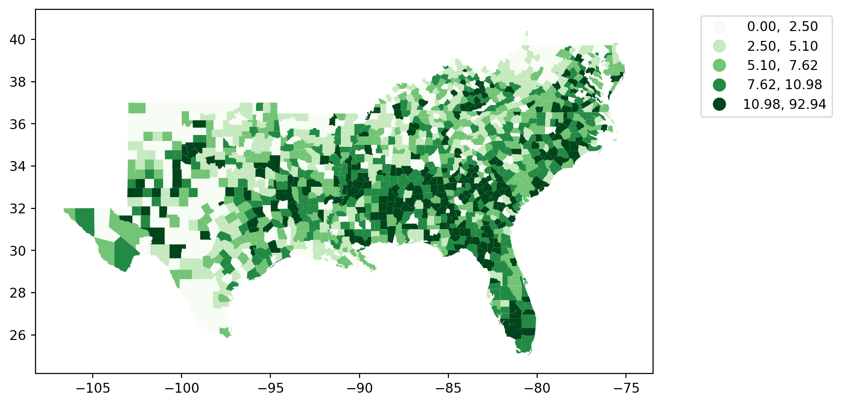
Change the color map: Multiple Hues
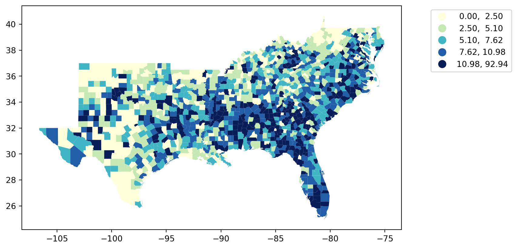
Diverging Color Map
Alternative Diverging Color Map
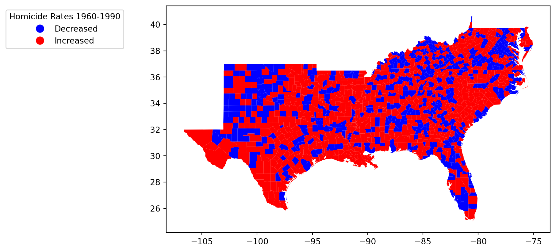
Qualitative Color Scheme
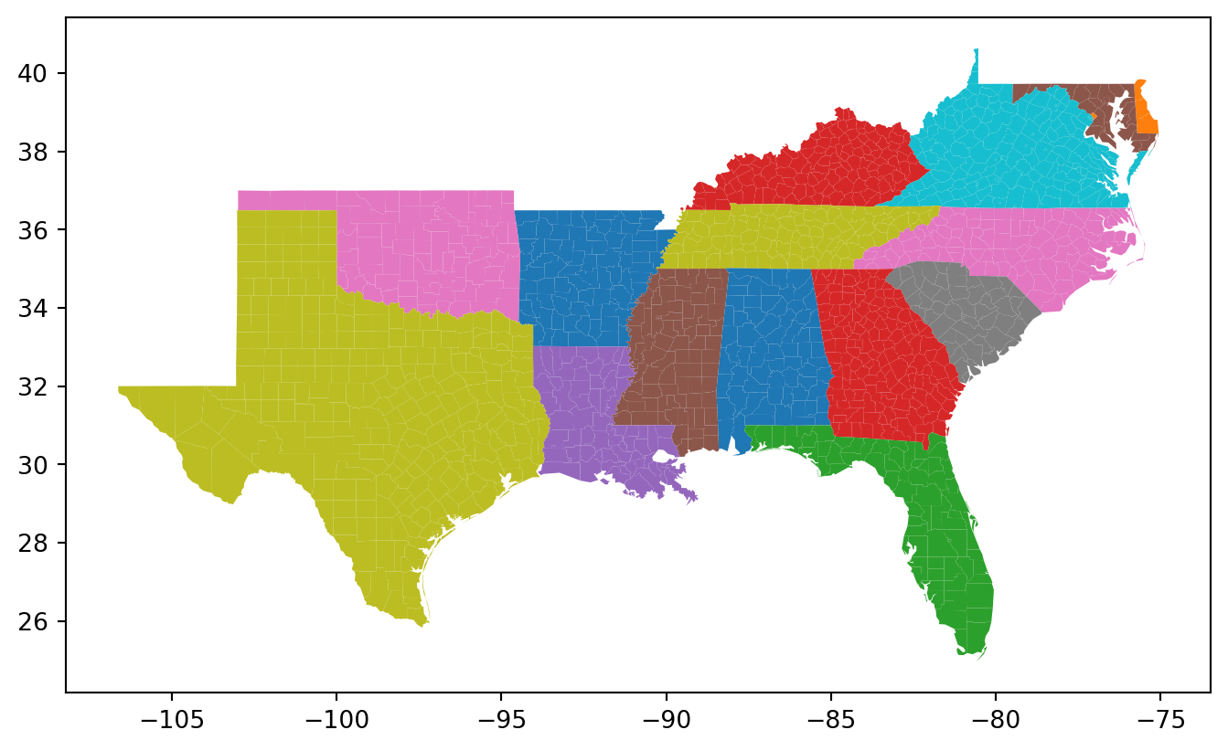
Qualitative Color Scheme
Qualitative Color Scheme
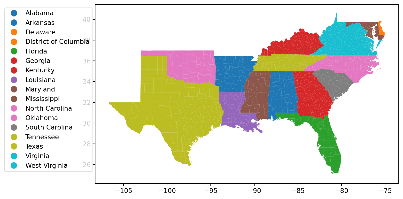
Qualitative Color Scheme
Deciles
Maximum Breaks
Fisher Jenks


Statistical Fit

Questions