Clustering and Regionalization in Geographic Data Science

Clustering

What is Clustering?

  • Definition: Grouping observations based on multivariate similarity.
  • Purpose: Simplify complex, multidimensional data into clusters.
  • Applications:
    • Geodemographic clusters in San Diego Census tracts.
    • Socioeconomic analysis using clustering.

How Clustering Works

  1. Unsupervised Learning: No labels, groups based on similarity.
  2. Multivariate Processes: Clusters represent similarities in many variables.
  3. Profile Creation: Simplifies the interpretation of complex data.

Example: Socioeconomic clustering

import pandas as pd
import geopandas as gpd
from sklearn.cluster import KMeans
from sklearn.preprocessing import StandardScaler

# Example dataset (San Diego tracts)
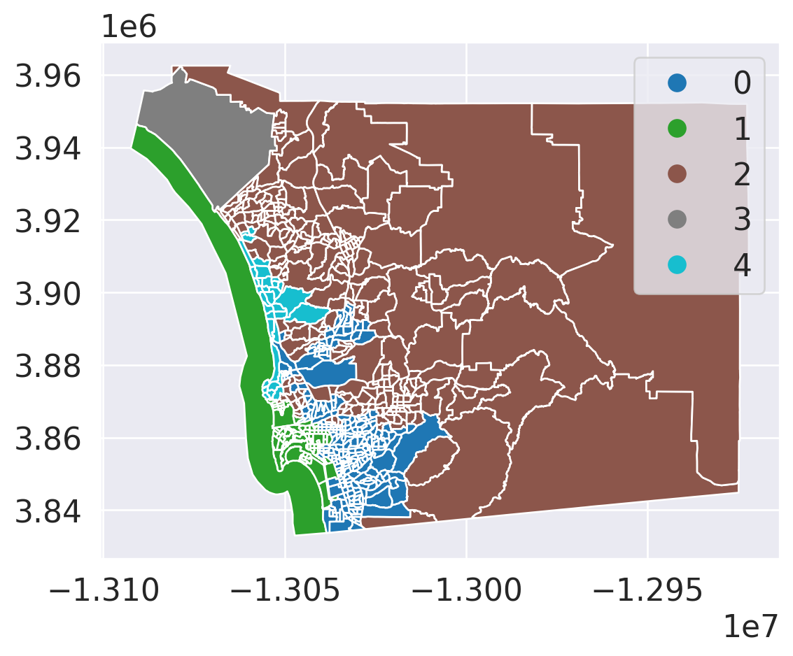
data = gpd.read_file('~/data/385/sandiego_tracts.gpkg')

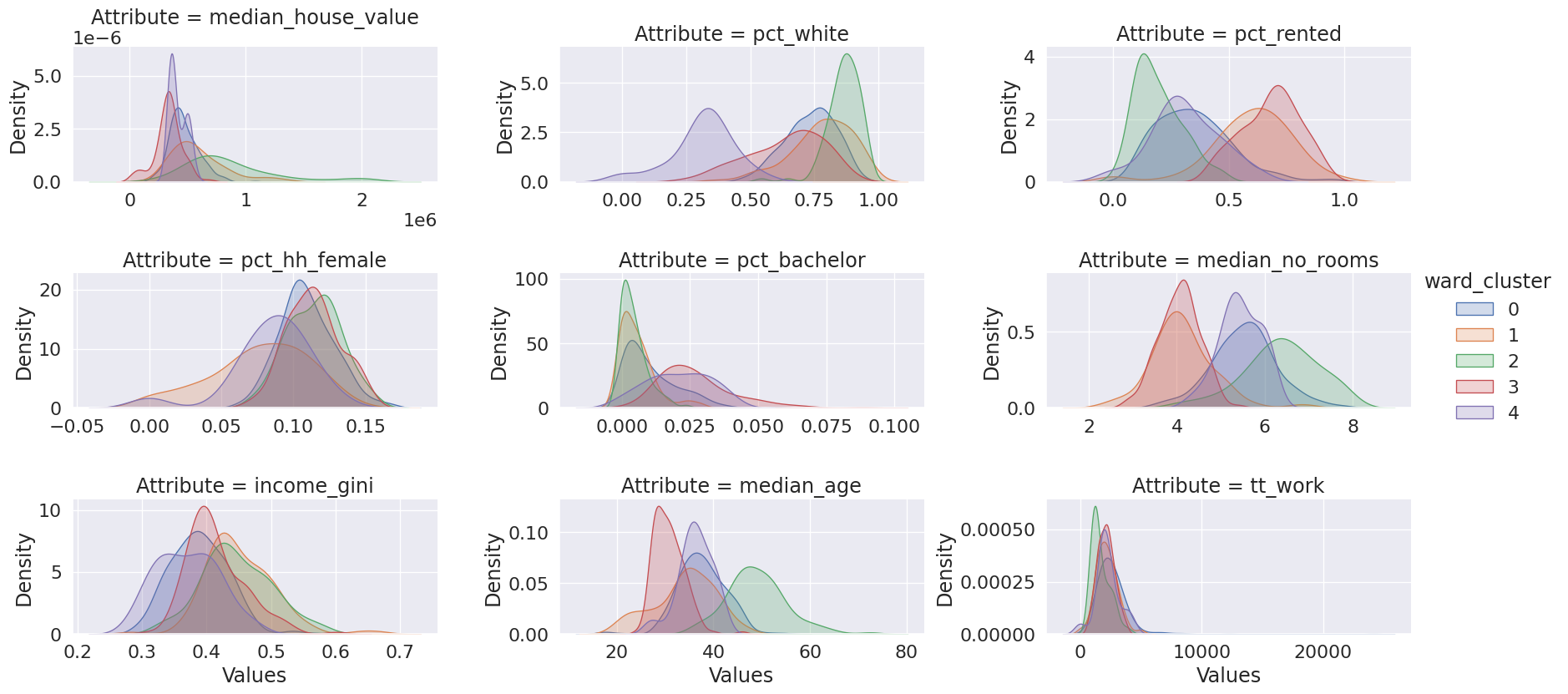
# Select clustering variables
cluster_variables = ["median_house_value", "pct_white", "pct_rented", "pct_hh_female", "pct_bachelor", "median_no_rooms", "income_gini", "median_age", "tt_work"]
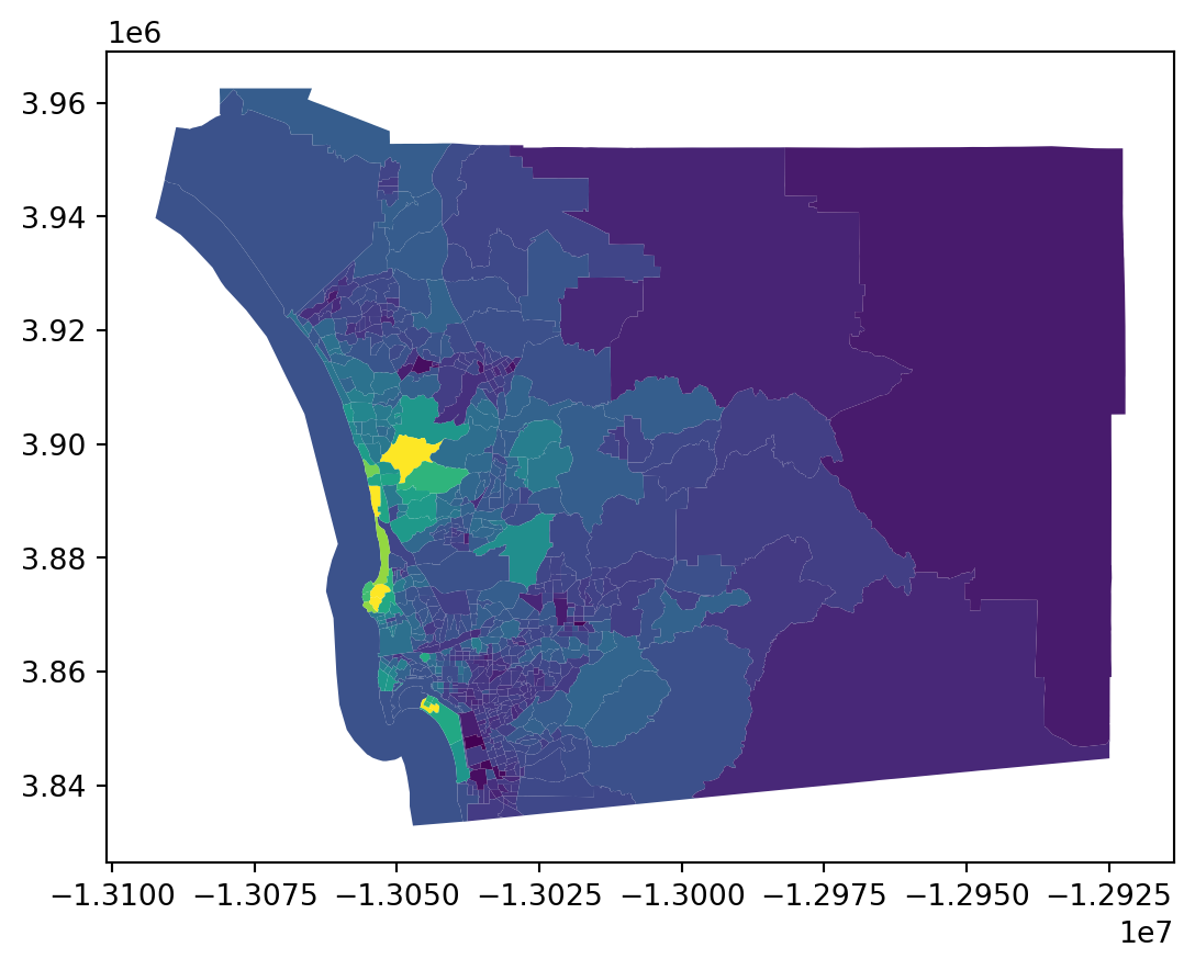
data.plot('median_house_value')

Data Preparation: Scaling

data[cluster_variables[0:3]].head()
median_house_value pct_white pct_rented
0 732900.000000 0.916988 0.373913
1 473800.000000 0.790558 0.205144
2 930600.000000 0.880250 0.279029
3 478500.000000 0.800598 0.196512
4 515570.896382 0.753799 0.949887

Data Preparation: Scaling

# Scale the data
scaler = StandardScaler()
scaled_data = scaler.fit_transform(data[cluster_variables])
scaled_data[0:5, 0:3]
array([[ 8.12429126e-01,  1.23188973e+00, -2.41143211e-01],
       [-1.56149785e-01,  4.51803106e-01, -9.86504682e-01],
       [ 1.55147988e+00,  1.00521260e+00, -6.60192373e-01],
       [-1.38580040e-01,  5.13751652e-01, -1.02462658e+00],
       [-2.17594415e-16,  2.25001983e-01,  2.30262050e+00]])

KMeans

# Run KMeans
kmeans = KMeans(n_clusters=5, random_state=0)
data['kmeans_cluster'] = kmeans.fit_predict(scaled_data)

# Visualize clusters
data.plot(column='kmeans_cluster', categorical=True, legend=True)

Ward’s Hierarchical Clustering

  • Definition: Agglomerative clustering method.
  • Steps:
    1. Start with each observation as its own cluster.
    2. Merge clusters based on proximity.
    3. Create a hierarchy of clustering solutions.
  • Application: Socioeconomic clusters of San Diego.

Example: Ward’s Method

from sklearn.cluster import AgglomerativeClustering

# Perform Ward's hierarchical clustering
ward = AgglomerativeClustering(n_clusters=5, linkage="ward")
data['ward_cluster'] = ward.fit_predict(scaled_data)

# Visualize Ward clusters
data.plot(column='ward_cluster', categorical=True, legend=True)

import matplotlib.pyplot as plt
from scipy.cluster.hierarchy import dendrogram, linkage
Z = linkage(scaled_data, method='ward')
plt.figure(figsize=(8, 5))
plt.title("Dendrogram for Ward's Hierarchical Clustering")
dendrogram(Z)
plt.show()

Cluster Profile: Data Setup

tidy_db = data.set_index('ward_cluster')
tidy_db = tidy_db[cluster_variables]
tidy_db = tidy_db.stack()
tidy_db = tidy_db.reset_index()
tidy_db = tidy_db.rename(
    columns={"level_1": "Attribute", 0: "Values"})
tidy_db.head()
ward_cluster Attribute Values
0 1 median_house_value 732900.000000
1 1 pct_white 0.916988
2 1 pct_rented 0.373913
3 1 pct_hh_female 0.052896
4 1 pct_bachelor 0.000000

import seaborn
import matplotlib.pyplot as plt

seaborn.set(font_scale=1.5)
# Setup the facets
facets = seaborn.FacetGrid(
    data=tidy_db,
    col="Attribute",
    hue="ward_cluster",
    sharey=False,
    sharex=False,
    aspect=2,
    col_wrap=3,
);
# Build the plot from `sns.kdeplot`
_ = facets.map(seaborn.kdeplot, "Values", shade=True).add_legend();
facets.savefig("facets.png")
plt.close()

Cluster Profiles

Spatial Autocorrelation and Clustering

from esda.moran import Moran
from libpysal.weights import Queen

# Create spatial weights matrix
w = Queen.from_dataframe(data)

# Moran's I for a variable
mi = Moran(data['median_house_value'], w)
print(mi.I, mi.p_sim)
0.6466184001197568 0.001

Regionalization

What is Regionalization?

  • Definition: Clustering with geographic constraints.
  • Importance: Ensures clusters are both statistically and spatially coherent.

Spatial Weights in Regionalization

  • Spatial Weights Matrix: Defines connectivity (e.g., Queen contiguity, K-nearest neighbors).

Example: Spatially Constrained Clustering

from libpysal.weights import Queen

# Use spatial weights to constrain clustering
wq = Queen.from_dataframe(data)
ward_spatial = AgglomerativeClustering(n_clusters=5, linkage="ward",
                                       connectivity=wq.sparse)
data['ward_spatial_cluster'] = ward_spatial.fit_predict(scaled_data)
data.plot(column='ward_spatial_cluster', categorical=True, legend=True)

Clusters versus Regions

Clusters versus Regions

  • Connected Component: a subgraph in which any two vertices are connected to each other by paths.
  • Regions: formed as connected components defined on the spatial adjacency graph
  • Multivariate Clusters: may or may not be spatially connected components

Connected Components

Ward Cluster Graph

import libpysal
gc = libpysal.graph.Graph.build_block_contiguity(data.ward_cluster)
gc.summary()
Graph Summary Statistics
Number of nodes: 628
Number of edges: 114490
Number of connected components: 5
Number of isolates: 0
Number of non-zero edges: 114490
Percentage of non-zero edges: 29.03%
Number of asymmetries: NA
Sum of weights and Traces
S0: 114490 GG: 114490
S1: 228980 G'G: 114490
S3: 106484296 G'G + GG: 228980
Graph indexed by: [0, 5, 9, 10, 13, ...]

Spatial Ward Cluster Graph

gcs = libpysal.graph.Graph.build_block_contiguity(data.ward_spatial_cluster)
gcs.summary()
Graph Summary Statistics
Number of nodes: 628
Number of edges: 142610
Number of connected components: 5
Number of isolates: 1
Number of non-zero edges: 142610
Percentage of non-zero edges: 36.16%
Number of asymmetries: NA
Sum of weights and Traces
S0: 142610 GG: 142610
S1: 285220 G'G: 142610
S3: 144306296 G'G + GG: 285220
Graph indexed by: [0, 1, 3, 7, 12, ...]

Queen Graph

import libpysal
gq  = libpysal.graph.Graph.from_W(wq)
gq.summary()
Graph Summary Statistics
Number of nodes: 628
Number of edges: 4016
Number of connected components: 1
Number of isolates: 0
Number of non-zero edges: 4016
Percentage of non-zero edges: 1.02%
Number of asymmetries: NA
Sum of weights and Traces
S0: 4016 GG: 4016
S1: 8032 G'G: 4016
S3: 113728 G'G + GG: 8032
Graph indexed by: [0, 1, 2, 3, 4, ...]

Intersection Graph (Queen + Ward )

import libpysal
gcq_int = gq.intersection(gc)
gcq_int.summary()
Graph Summary Statistics
Number of nodes: 628
Number of edges: 2208
Number of connected components: 80
Number of isolates: 33
Number of non-zero edges: 2208
Percentage of non-zero edges: 0.57%
Number of asymmetries: NA
Sum of weights and Traces
S0: 2208 GG: 2208
S1: 4416 G'G: 2208
S3: 41312 G'G + GG: 4416
Graph indexed by: [0, 1, 2, 3, 4, ...]

Intersection Graph (Queen + Ward Spatial)

import libpysal
gcsq_int = gq.intersection(gcs)
gcsq_int.summary()
Graph Summary Statistics
Number of nodes: 628
Number of edges: 3394
Number of connected components: 5
Number of isolates: 1
Number of non-zero edges: 3394
Percentage of non-zero edges: 0.86%
Number of asymmetries: NA
Sum of weights and Traces
S0: 3394 GG: 3394
S1: 6788 G'G: 3394
S3: 83704 G'G + GG: 6788
Graph indexed by: [0, 1, 2, 3, 4, ...]

Code
import matplotlib.pyplot as plt

fig, axes = plt.subplots(1,2, figsize=(12,6))
data.plot(column='ward_cluster', categorical=True, ax=axes[0], linewidth=0.1)
axes[0].set_title('Ward')
axes[0].axis('off')
data.plot(column='ward_spatial_cluster', categorical=True, ax=axes[1], linewidth=0.1, legend=True,
          legend_kwds={'bbox_to_anchor': (1.3, 1),
                       'title': "Cluster"})
axes[1].set_title('Ward Spatial')
axes[1].axis('off')
plt.tight_layout()

Comparison

Method Clusters Regions
Ward 5 80
Spatial Ward 5 5

Conclusion

Recap of Key Points

  • Multivariate Clustering
  • Regionalization
  • Clusters versus Regions

Questions