Global Spatial Autocorrelation

Serge Rey

Outline

• Spatial Autocorrelation
• Testing for Global Autocorrelation
• Join Counts
• Moran’s I
• Conclusion

Spatial Autocorrelation

Tobler’s First Law of Geography

Everything is related to everything else, but near things are more related than distant things.

Waldo Tobler

TFL: Blessing or Curse?

Sources of Spatial Variation

• Compositional Influences

  • Disease rates may reflect differences in age structure
  • Economic growth rates may reflect differences in industrial composition

• Contextual Influences

  • Disease rates may be due to exposure to pollutants
  • Economic growth may be due to differences in local labor markets/institutions

Contextual Effects

• Spillovers

  • housing values
  • retail price behavior
  • policy copy-catting

• Contagion

  • infectious disease spread
  • peer influences/networks
  • neighborhoods provide role models

Objectives of Areal Data Analysis

• Infer whether there are a spatial trend or pattern in the attribute values recorded over the sub-regions
• First order variation: Trend in the mean
• Second order variation: Spatial dependence

Trend in the mean

from geosnap import DataStore
import geopandas as gpd

datasets = DataStore()

from geosnap.io import get_acs
ca = get_acs(datasets, state_fips=['06'], level='tract', years=[2016])
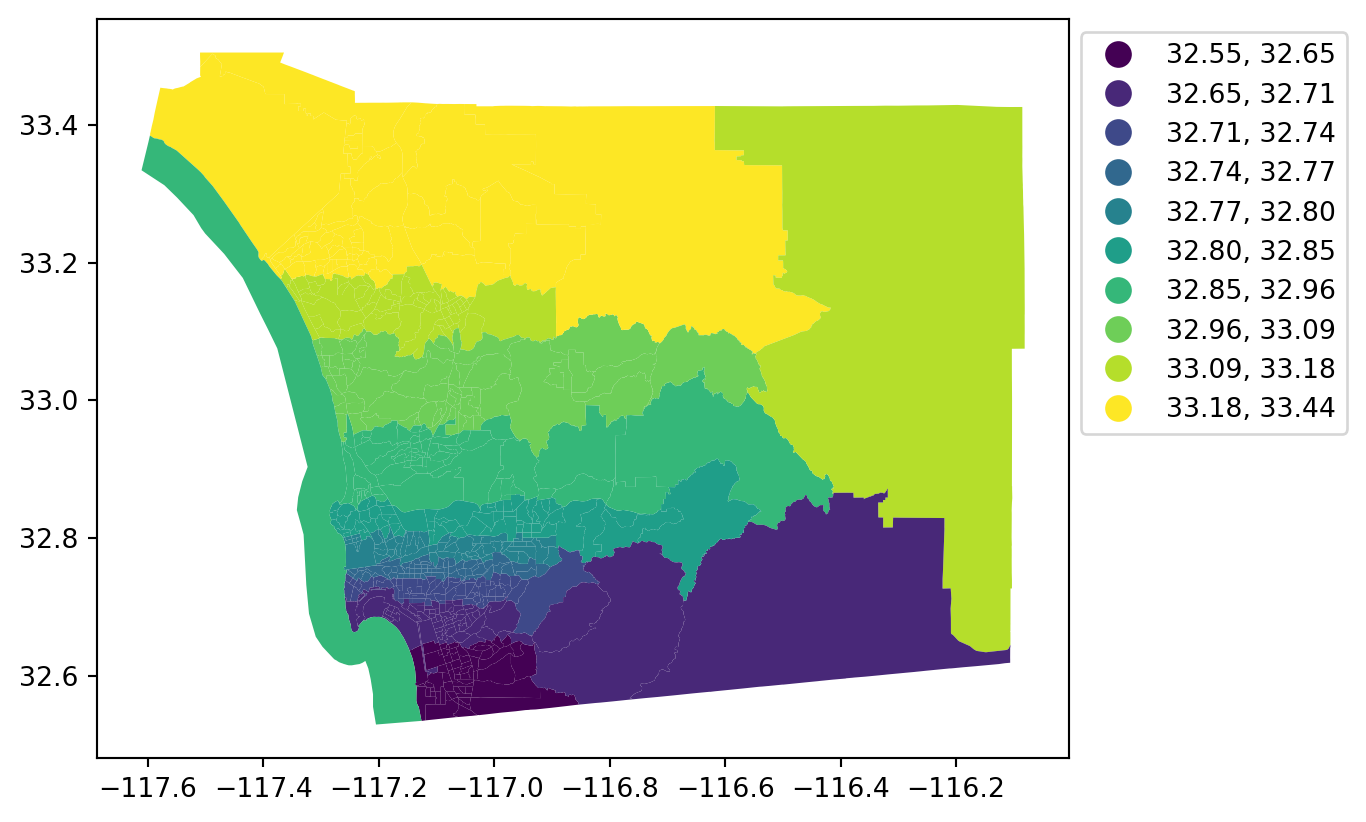
sd = ca[ca.geoid.str.startswith('06073')]
sd['lat'] = sd.geometry.centroid.y
sd.plot('lat', scheme='quantiles', k=10, legend=True,
        legend_kwds={'bbox_to_anchor': (1.3,1)});

Second order variation

sd['p_poverty_rate'] = sd.p_poverty_rate.fillna(0)
sd.plot(column='p_poverty_rate', scheme='quantiles', k=10, legend=True,
        legend_kwds={'bbox_to_anchor': (1.3,1)});

Spatial Dependence

Categorizing

• Type: Substantive versus nuisance

• Direction: Positive versus negative

Issues

• Time versus space

• Inference

Substantive Spatial Dependence

Process Based

• Part of the process under study

• Leaving it out

  • Incomplete understanding

  • Biased inferences

Nuisance Spatial Dependence

Not Process Based

• Artifact of data collection

• Process boundaries not matching data boundaries

• Scattering across pixels

• GIS induced

Boundary

Boundary Mismatch

• Even if \(A\) and \(B\) are independent

• \(A'\) and \(B'\) will be dependent

Nusiance vs. Substantive Dependence

Issues

• Not always easy to differentiate from substantive

• Different implications for each type

• Specification strategies (Econometrics)

• Both can be operating jointly

Space versus Time

Temporal Dependence

• Past influences the future

• Recursive

• One dimension

Space versus Time

Spatial Dependence

• Multi-directional

• Simultaneous

Testing for Global Autocorrelation

Hypotheses

• Null Hypothesis (\(H_o\))
• Alternative Hypothesis (\(H_a\))

Null Hypothesis (\(H_o\))

• observed spatial pattern of values is equally likely as any other spatial pattern
• values at one location do no depend on values at other (neighboring) locations
• under spatial randomness, the location of values may be altered without affecting the information content of the data

Alternative Hypothesis (\(H_a\))

• there is spatial autocorrelation in the data, indicating that the values of the variable are not randomly distributed over space, but instead exhibit some for of spatial dependence.
• p-value = probability of getting such a pattern from a spatially random process
• p-value != probability the process is random

Forms of Spatial Autocorrelation

Positive Spatial Autocorrelation

Positive Spatial Autocorrelation

• Clustering: like values tend to be in similar locations

  • neighbor similarity
  • more alike than would be expected under spatial randomness

• Compatible with diffusion

  • but not necessarily caused by diffusion

Negative Spatial Autocorrelation

Negative Spatial Autocorrelation

• Anti-clustering

  • neighbor dissimilarity
  • more dissimilar than they would be under spatial randomness

• Compatible with competition

  • but not necessarily caused by competition

Spatial Autcorrelation Statistic

Structure

• Formal test of match between value similarity and locational similarity

• Statistic summarizes both aspects

• Significance

  • how likely is it (p-value) that the computed statistic would take this (extreme) value in a spatially random pattern

Join Counts

Binary Variable

high_poverty = sd.p_poverty_rate > sd.p_poverty_rate.median()
sd['high_poverty'] = high_poverty * 1
sd.plot(column='high_poverty', categorical=True, legend=True,
        edgecolor='k')

Explore

sd.explore(column='p_poverty_rate', legend=True,
           tooltip=['high_poverty', 'p_poverty_rate', 'geoid'])

Make this Notebook Trusted to load map: File -> Trust Notebook

Spatial Joins

from esda.join_counts import Join_Counts
from libpysal.weights import Queen
w = Queen.from_dataframe(sd)

Joins

w.s0 

4018.0

\[w.s0 = \sum_i \sum_j w_{i,j}\]

• Number of non-zero values in \(w\)
• 2x the number of joins

Neighbors

import numpy as np
sd['neighbors'] = np.array(list(w.cardinalities.values()))

sd.explore(column='p_poverty_rate', legend=True, 
           tooltip=['high_poverty', 'p_poverty_rate', 'geoid', 'neighbors']) 

Make this Notebook Trusted to load map: File -> Trust Notebook

Spatial Lag

\(L_i = \sum_{j} w_{i,j} B_j\)

• the spatial lag is the number of B neighbors
• if the focal unit is B, then it involved in as many BB joins as it has B neighbors
• if the focal unit is W(hite), it is involved in 0 BB joins

Spatial Lag

from libpysal.weights import lag_spatial
sd['BNeighbors'] = lag_spatial(w, sd.high_poverty)
sd.explore(column='p_poverty_rate', legend=True, 
           tooltip=['high_poverty', 'p_poverty_rate', 'geoid',
                    'neighbors', 'BNeighbors']) 

Make this Notebook Trusted to load map: File -> Trust Notebook

Join Counts

from esda.join_counts import Join_Counts
from libpysal.weights import Queen
import numpy as np
np.random.seed(12345)
w = Queen.from_dataframe(sd)
jc = Join_Counts(sd.high_poverty, w)
jc.bb, jc.bw, jc.ww

(660.0, 667.0, 682.0)

\(BB =\frac{1}{2} \sum_i \sum_j w_{i,j} B_i B_j = \frac{1}{2} \sum_i B_i L_i\)

Join Counts Inference

jc.p_sim_bb, jc.mean_bb, jc.bb

(0.001, 502.2142142142142, 660.0)

Moran’s I

Moran’s I

\[ I = \dfrac{n}{\sum_i\sum_j w_{ij}} \dfrac{\sum_i\sum_j w_{i,j} \, z_i \, z_j}{\sum_i z_i^2} \]

• \(z_i = y_i - \bar{y}\)
• \(\sum_i \sum_j w_{i,j}z_i z_j = \sum_i z_i \sum_j w_{i,j} z_j = \sum_i z_i l_i\)

Moran’s I

from esda.moran import Moran
from libpysal.weights import Queen
np.random.seed(12345)
mc = Moran(sd.p_poverty_rate, w, transformation='r')
mc.I, mc.EI, mc.p_norm, mc.p_sim

(0.5345296697872074, -0.001594896331738437, 1.1152317274459047e-123, 0.001)

Conclusion

Recap of Key Points

• Spatial Autocorrelation
• Join Counts
• Moran’s I

Questions