Methods for Area Unit Data
Introduction
What is Area Unit Data?
- Analysis of data associated with spatial zones or areas
- Areas may be regular in shape and size, or irregular
Focus in Area Unit Data Analysis
- Variation in an attribute across our spatial units
- The spatial variation is not continuous
- Spatial units are polygons
- variation across polygons
- no variation within polygons
Notation
Our substantive attribute of interest is \(Y\).
Our process is represented as:
\[ \{ Y(A_i), \ A_i \in A_1, A_2, \ldots, A_n \} \]
\[ A_1 \cup A_2 \cup \ldots \cup A_n = {R} \]
- \(Y(A_i)\) is a set of random variables indexed by sub-regions
- \(A_1, A_2, \ldots , A_n\) are sub-regions of \({R}\)
Areal Unit Data (Lattice)
Spatial Domain: \({R}\)
Discrete and fixed
Locations nonrandom
Locations countable
Examples of lattice data
Attributes collected by ZIP code
census tract
Lattice Data: Indexing
Site
Each location is now an area or site
One observation on \(Y\) for each site
Need a spatial index: \(Y(s_i)\)
\(Y(s_i)\)
\(s_i\) is a representative location within the site
e.g., centroid, largest city
Allows for measuring distances between sites
Lattice Data: County Per Capita Incomes
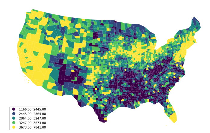
1969
Objectives
- Infer whether there are a spatial trend or pattern in the attribute values recorded over the sub-regions
- First order variation: Trend in the mean
- Second order variation: Spatial dependence
Visualizing Area Unit Data
Choropleths
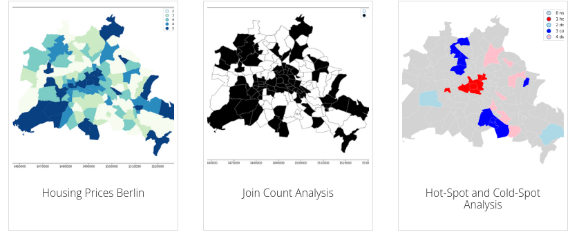
Interactivity
Analyzing Area Unit Data
Spatial Dependence
Hell might be a world without spatial dependence since it would be impossible to live there in any practical and meaningful way.
Spatial Autocorrelation
- Definition: The degree to which objects close to each other in space are also similar in other attributes.
- Examples: Clustered patterns of disease, similar land uses in neighboring areas.
- Measurement: Moran’s I, Geary’s C.
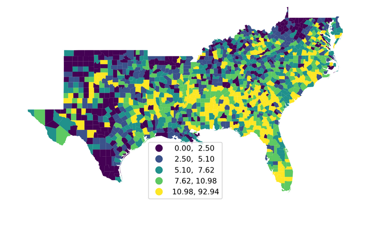
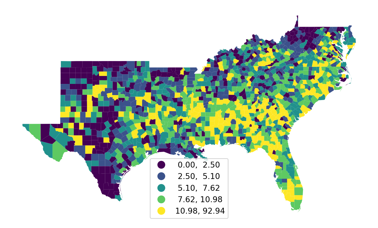
Spatial Autocorrelation (Homicide Rates 1969)
Area Unit Data in Python
Imports
Loading an example data set
Finding out about the example
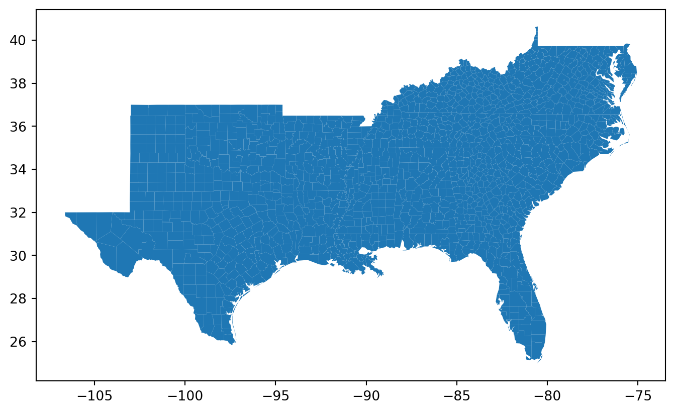
Creating a GeoDataFrame from a file
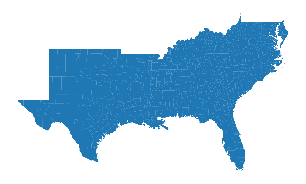
Plotting the geometries
Checking the Coordinate Reference System
<Geographic 2D CRS: EPSG:4326>
Name: WGS 84
Axis Info [ellipsoidal]:
- Lat[north]: Geodetic latitude (degree)
- Lon[east]: Geodetic longitude (degree)
Area of Use:
- name: World.
- bounds: (-180.0, -90.0, 180.0, 90.0)
Datum: World Geodetic System 1984 ensemble
- Ellipsoid: WGS 84
- Prime Meridian: GreenwichTurning of the axis
Inspecting the GDF
Inspecting the GeoSeries
0 POLYGON ((-80.62805 40.39816, -80.60204 40.480...
1 POLYGON ((-80.52625 40.16245, -80.5876 40.1750...
2 POLYGON ((-80.52517 40.02275, -80.73843 40.035...
3 POLYGON ((-80.52447 39.72113, -80.83248 39.718...
4 POLYGON ((-75.7727 39.38301, -75.79144 39.7237...
...
1407 POLYGON ((-79.14433 36.54606, -79.21706 36.549...
1408 POLYGON ((-79.43775 37.61596, -79.45834 37.603...
1409 POLYGON ((-80.12475 37.1251, -80.14045 37.1283...
1410 POLYGON ((-76.39569 37.10771, -76.4027 37.0905...
1411 POLYGON ((-77.53178 38.56506, -77.72094 38.840...
Name: geometry, Length: 1412, dtype: geometryInspecting the Columns
Index(['NAME', 'STATE_NAME', 'STATE_FIPS', 'CNTY_FIPS', 'FIPS', 'STFIPS',
'COFIPS', 'FIPSNO', 'SOUTH', 'HR60', 'HR70', 'HR80', 'HR90', 'HC60',
'HC70', 'HC80', 'HC90', 'PO60', 'PO70', 'PO80', 'PO90', 'RD60', 'RD70',
'RD80', 'RD90', 'PS60', 'PS70', 'PS80', 'PS90', 'UE60', 'UE70', 'UE80',
'UE90', 'DV60', 'DV70', 'DV80', 'DV90', 'MA60', 'MA70', 'MA80', 'MA90',
'POL60', 'POL70', 'POL80', 'POL90', 'DNL60', 'DNL70', 'DNL80', 'DNL90',
'MFIL59', 'MFIL69', 'MFIL79', 'MFIL89', 'FP59', 'FP69', 'FP79', 'FP89',
'BLK60', 'BLK70', 'BLK80', 'BLK90', 'GI59', 'GI69', 'GI79', 'GI89',
'FH60', 'FH70', 'FH80', 'FH90', 'geometry'],
dtype='object')Interactive Map
Describing a column
Static Choropleth: HR60
How many states are there in this dataset
How many counties?
How many counties in each state?
| NAME | STATE_FIPS | CNTY_FIPS | FIPS | STFIPS | COFIPS | FIPSNO | SOUTH | HR60 | HR70 | ... | BLK90 | GI59 | GI69 | GI79 | GI89 | FH60 | FH70 | FH80 | FH90 | geometry | |
|---|---|---|---|---|---|---|---|---|---|---|---|---|---|---|---|---|---|---|---|---|---|
| STATE_NAME | |||||||||||||||||||||
| Alabama | 67 | 67 | 67 | 67 | 67 | 67 | 67 | 67 | 67 | 67 | ... | 67 | 67 | 67 | 67 | 67 | 67 | 67 | 67 | 67 | 67 |
| Arkansas | 75 | 75 | 75 | 75 | 75 | 75 | 75 | 75 | 75 | 75 | ... | 75 | 75 | 75 | 75 | 75 | 75 | 75 | 75 | 75 | 75 |
| Delaware | 3 | 3 | 3 | 3 | 3 | 3 | 3 | 3 | 3 | 3 | ... | 3 | 3 | 3 | 3 | 3 | 3 | 3 | 3 | 3 | 3 |
| District of Columbia | 1 | 1 | 1 | 1 | 1 | 1 | 1 | 1 | 1 | 1 | ... | 1 | 1 | 1 | 1 | 1 | 1 | 1 | 1 | 1 | 1 |
| Florida | 67 | 67 | 67 | 67 | 67 | 67 | 67 | 67 | 67 | 67 | ... | 67 | 67 | 67 | 67 | 67 | 67 | 67 | 67 | 67 | 67 |
| Georgia | 159 | 159 | 159 | 159 | 159 | 159 | 159 | 159 | 159 | 159 | ... | 159 | 159 | 159 | 159 | 159 | 159 | 159 | 159 | 159 | 159 |
| Kentucky | 120 | 120 | 120 | 120 | 120 | 120 | 120 | 120 | 120 | 120 | ... | 120 | 120 | 120 | 120 | 120 | 120 | 120 | 120 | 120 | 120 |
| Louisiana | 64 | 64 | 64 | 64 | 64 | 64 | 64 | 64 | 64 | 64 | ... | 64 | 64 | 64 | 64 | 64 | 64 | 64 | 64 | 64 | 64 |
| Maryland | 24 | 24 | 24 | 24 | 24 | 24 | 24 | 24 | 24 | 24 | ... | 24 | 24 | 24 | 24 | 24 | 24 | 24 | 24 | 24 | 24 |
| Mississippi | 82 | 82 | 82 | 82 | 82 | 82 | 82 | 82 | 82 | 82 | ... | 82 | 82 | 82 | 82 | 82 | 82 | 82 | 82 | 82 | 82 |
| North Carolina | 100 | 100 | 100 | 100 | 100 | 100 | 100 | 100 | 100 | 100 | ... | 100 | 100 | 100 | 100 | 100 | 100 | 100 | 100 | 100 | 100 |
| Oklahoma | 77 | 77 | 77 | 77 | 77 | 77 | 77 | 77 | 77 | 77 | ... | 77 | 77 | 77 | 77 | 77 | 77 | 77 | 77 | 77 | 77 |
| South Carolina | 46 | 46 | 46 | 46 | 46 | 46 | 46 | 46 | 46 | 46 | ... | 46 | 46 | 46 | 46 | 46 | 46 | 46 | 46 | 46 | 46 |
| Tennessee | 95 | 95 | 95 | 95 | 95 | 95 | 95 | 95 | 95 | 95 | ... | 95 | 95 | 95 | 95 | 95 | 95 | 95 | 95 | 95 | 95 |
| Texas | 254 | 254 | 254 | 254 | 254 | 254 | 254 | 254 | 254 | 254 | ... | 254 | 254 | 254 | 254 | 254 | 254 | 254 | 254 | 254 | 254 |
| Virginia | 123 | 123 | 123 | 123 | 123 | 123 | 123 | 123 | 123 | 123 | ... | 123 | 123 | 123 | 123 | 123 | 123 | 123 | 123 | 123 | 123 |
| West Virginia | 55 | 55 | 55 | 55 | 55 | 55 | 55 | 55 | 55 | 55 | ... | 55 | 55 | 55 | 55 | 55 | 55 | 55 | 55 | 55 | 55 |
17 rows × 69 columns
Which state had the highest median county homicide rate in 1960?
| HR60 | |
|---|---|
| STATE_NAME | |
| Alabama | 9.623977 |
| Arkansas | 4.704111 |
| Delaware | 4.228385 |
| District of Columbia | 10.471807 |
| Florida | 9.970306 |
| Georgia | 9.300076 |
| Kentucky | 5.235436 |
| Louisiana | 6.840286 |
| Maryland | 5.335208 |
| Mississippi | 8.919274 |
| North Carolina | 7.633043 |
| Oklahoma | 4.269126 |
| South Carolina | 7.509437 |
| Tennessee | 4.877751 |
| Texas | 4.326215 |
| Virginia | 6.672004 |
| West Virginia | 2.623226 |
Which county had the highest maximum county homicide rate in 1960?
| HR60 | |
|---|---|
| STATE_NAME | |
| Alabama | 24.903499 |
| Arkansas | 21.154427 |
| Delaware | 7.286472 |
| District of Columbia | 10.471807 |
| Florida | 40.744262 |
| Georgia | 53.304904 |
| Kentucky | 37.250885 |
| Louisiana | 18.243736 |
| Maryland | 14.327234 |
| Mississippi | 24.833923 |
| North Carolina | 25.660127 |
| Oklahoma | 17.088175 |
| South Carolina | 23.345940 |
| Tennessee | 20.894275 |
| Texas | 92.936803 |
| Virginia | 23.575639 |
| West Virginia | 11.482375 |
Intra-state dispersion
| HR60 | |
|---|---|
| STATE_NAME | |
| Alabama | 4.742337 |
| Arkansas | 4.574625 |
| Delaware | 1.815562 |
| District of Columbia | NaN |
| Florida | 7.990692 |
| Georgia | 7.906488 |
| Kentucky | 6.354316 |
| Louisiana | 4.189146 |
| Maryland | 4.064360 |
| Mississippi | 4.972698 |
| North Carolina | 4.596952 |
| Oklahoma | 4.231132 |
| South Carolina | 4.018644 |
| Tennessee | 4.354979 |
| Texas | 8.223844 |
| Virginia | 4.826707 |
| West Virginia | 2.773659 |
| HR60 | |
|---|---|
| STATE_NAME | |
| Texas | 144.992919 |
| Kentucky | 96.815524 |
| West Virginia | 93.234007 |
| Arkansas | 81.223752 |
| Oklahoma | 81.114430 |
| Tennessee | 75.426226 |
| Georgia | 73.774440 |
| Maryland | 71.898559 |
| Florida | 68.252692 |
| Virginia | 66.924041 |
| Louisiana | 59.994571 |
| Mississippi | 57.457024 |
| North Carolina | 57.013871 |
| Alabama | 49.070812 |
| South Carolina | 48.083524 |
| Delaware | 34.966796 |
| District of Columbia | NaN |
Conclusion
Recap of Key Points
- Definition of Area Unit Data
- Objectives of Area Unit Data Analysis
- Area Unit Data in Python
Questions