GeoPandas

Geometries for Vector Spatial Data

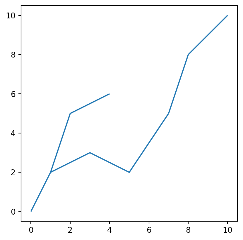
Earlier in the course we had a figure to illustrate vector spatial data:

This figure was built with the following code:

import matplotlib.pyplot as plt
from matplotlib.patches import Polygon as MplPolygon

# Data for streets (line strings)
streets = [
    [(0, 0), (1, 2), (3, 3)],
    [(3, 3), (5, 2), (7, 5)],
    [(7, 5), (8, 8), (10, 10)],
    [(1, 2), (2, 5), (4, 6)],
]

# Data for school catchments (polygons)
catchments = [
    [(0.5, 0.5), (2, 1), (1.5, 3), (0.5, 2)],
    [(3, 4), (5, 3.5), (6, 6), (4, 6.5)],
    [(7, 7), (8.5, 7.5), (9, 9), (7.5, 9)],
]

# Adjusting the data for one school per catchment
schools = [(1.2, 1.8), (4.7, 5.3), (8.2, 8.2)]

# Plotting the GIS map with one school per catchment
fig, ax = plt.subplots(figsize=(8, 8))

# Plotting the streets with one legend entry
ax.plot(*zip(*streets[0]), color='blue', linewidth=2, label="Streets")
for street in streets[1:]:
    street_x, street_y = zip(*street)
    ax.plot(street_x, street_y, color='blue', linewidth=2)

# Plotting the catchments with legend
for i, catchment in enumerate(catchments):
    polygon = MplPolygon(catchment, closed=True, color='orange', alpha=0.5, edgecolor='black')
    ax.add_patch(polygon)
    if i == 0:
        polygon.set_label("School Catchments")

# Plotting the schools (points) with one per catchment
school_x, school_y = zip(*schools)
ax.scatter(school_x, school_y, color='green', s=100, label="Schools")

# Set the legend and title
ax.legend()
ax.set_title('Vector GIS: Street Network, School Catchments, and Schools')
ax.set_xlim(-1, 11)
ax.set_ylim(-1, 11)
ax.set_aspect('equal')

# Save the figure to a file
plt.savefig("vector.png", dpi=300)

# Show the plot
plt.show()

/tmp/ipykernel_15976/1512531908.py:33: UserWarning: Setting the 'color' property will override the edgecolor or facecolor properties.
  polygon = MplPolygon(catchment, closed=True, color='orange', alpha=0.5, edgecolor='black')

Here, we are faking it regarding a GIS, as matplotlib is a visualization library and doesn’t actually allow us to do any spatial analysis per se.

Fortunately, there are a number of Python packages that are designed to wrangle spatial data:

shapely
GeoPandas

shapely

Shapely (shapely2007?) is a Python package for the manipulation and analysis of planar geometric objects.

We can use shapely to build up our example, starting with its Point class:

from shapely import Point

The Point class can be used to create instances for each of our schools, here using a python list comprehension:

school_points = [Point(school) for school in schools]

This results in a python list containing three shapely point objects:

school_points

[<POINT (1.2 1.8)>, <POINT (4.7 5.3)>, <POINT (8.2 8.2)>]

If we ask for the first point, we get a rendered point.

school_points[0]

And, if we unpack the list into individual points, we should see similar behavior.

school_0, school_1, school_2 = school_points

school_0

school_1

school_2

Just like we did for points, we can rely on shapely for dealing with our catchments, but this time using the Polygon class:

from shapely import Polygon

catchment_polygons = [Polygon(catchment) for catchment in catchments]

catchment_0, catchment_1, catchment_2 = catchment_polygons

catchment_0

catchment_1

catchment_2

And, finally, we can model the road network using the LineString class:

from shapely import LineString

street_lines = [LineString(street) for street in streets]

street_0, street_1, street_2, street_3 = street_lines

street_0

street_1

street_2

street_3

shapely Geometry Types

school_0.geom_type

'Point'

school_2.geom_type

'Point'

Points are zero-dimensional geometries, and thus have 0 area and 0 length:

school_0.area

0.0

school_0.length

0.0

list(school_0.coords)

[(1.2, 1.8)]

list(school_2.coords)

[(8.2, 8.2)]

LineStrings are one-dimensional geometric objects, having length but 0 area

street_1.length

5.841619252963779

street_1.area

0.0

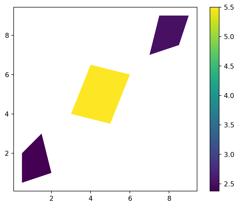
Finally, Polygons are two-dimensional geometric objects, having area:

catchment_1.area

5.5

as well as length:

catchment_1.length

9.508270432752164

geometry methods and spatial predicates

The power of these geometries comes from the functions and abilities to evaluate spatial predicates. These give us the building blocks of GIS operations for vector spatial data:

To see this, we can call the distance method of school_0 to determine the distance separating it from school_2:

school_0.distance(school_2)

9.4847245611035

We can also measure the difference between objects of different geometry types:

street_1.geom_type

'LineString'

school_0.distance(street_1)

2.1633307652783933

catchment_0.geom_type

'Polygon'

catchment_0.area

2.375

list(catchment_0.exterior.coords)

[(0.5, 0.5), (2.0, 1.0), (1.5, 3.0), (0.5, 2.0), (0.5, 0.5)]

catchment_0.bounds

(0.5, 0.5, 2.0, 3.0)

school_0.distance(catchment_0)

0.0

catchment_0.contains(school_0)

True

catchment_0.contains(school_1)

False

school_1.distance(catchment_0)

3.9408120990476063

Note

All the area, distance, and other measurements done with shapely objects utilize Cartesian coordinates.

GeoPandas

GeoPandas (kelsey_jordahl_2020_3946761?) is a python package that makes working with geospatial data easier. It relies on shapely and other libraries to extend the datatypes used by Pandas to allow spatial operations on geometric types.

The two important classes in GeoPandas are:

GeoSeries
GeoDataFrame

These are spatial extensions of the Series and DataFrame classes from pandas.

import and aliasing

import geopandas as gpd

GeoSeries

A GeoSeries is essentially a pandas Series object designed to store shapely geometry types:

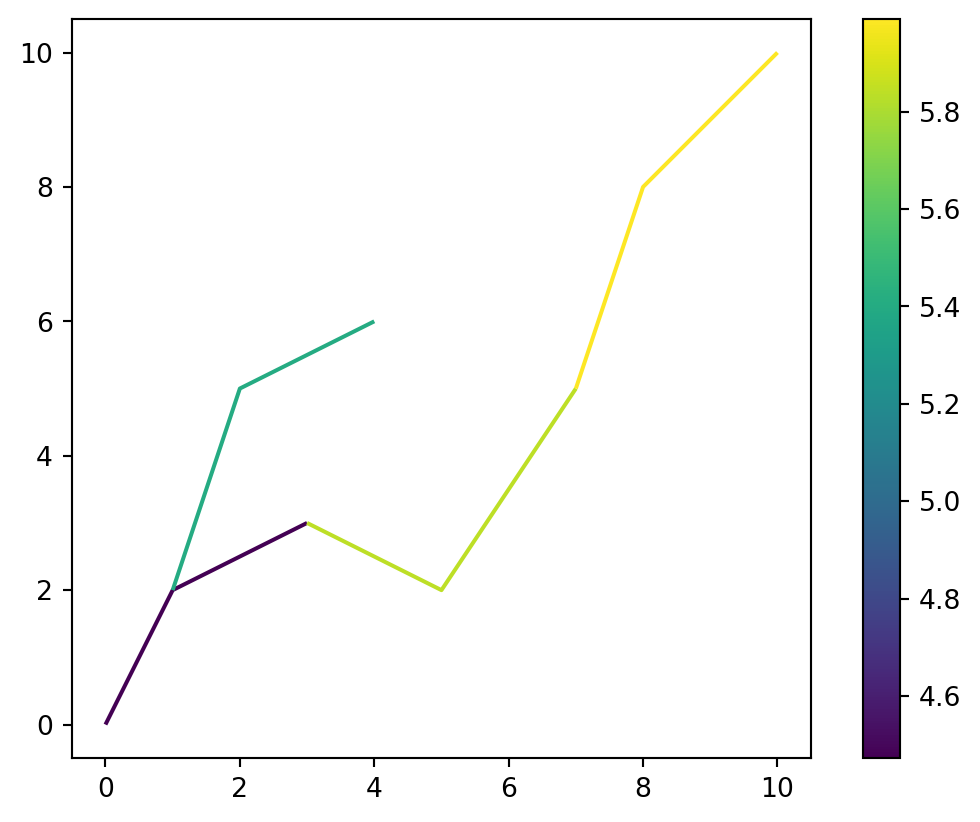
streets = gpd.GeoSeries(street_lines)

streets.plot()

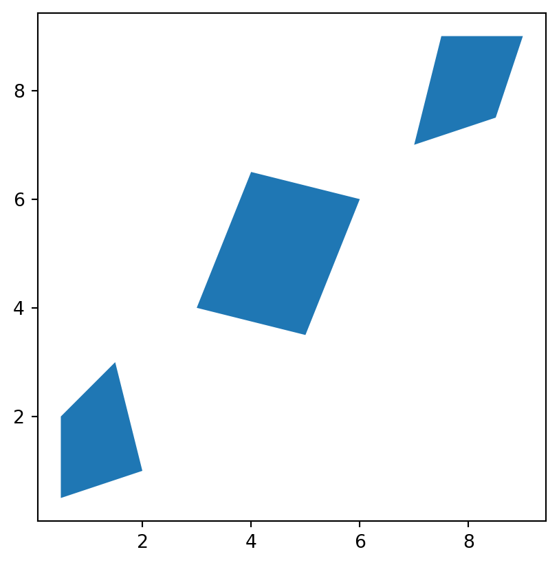
catchments = gpd.GeoSeries(catchment_polygons)

catchments.plot()

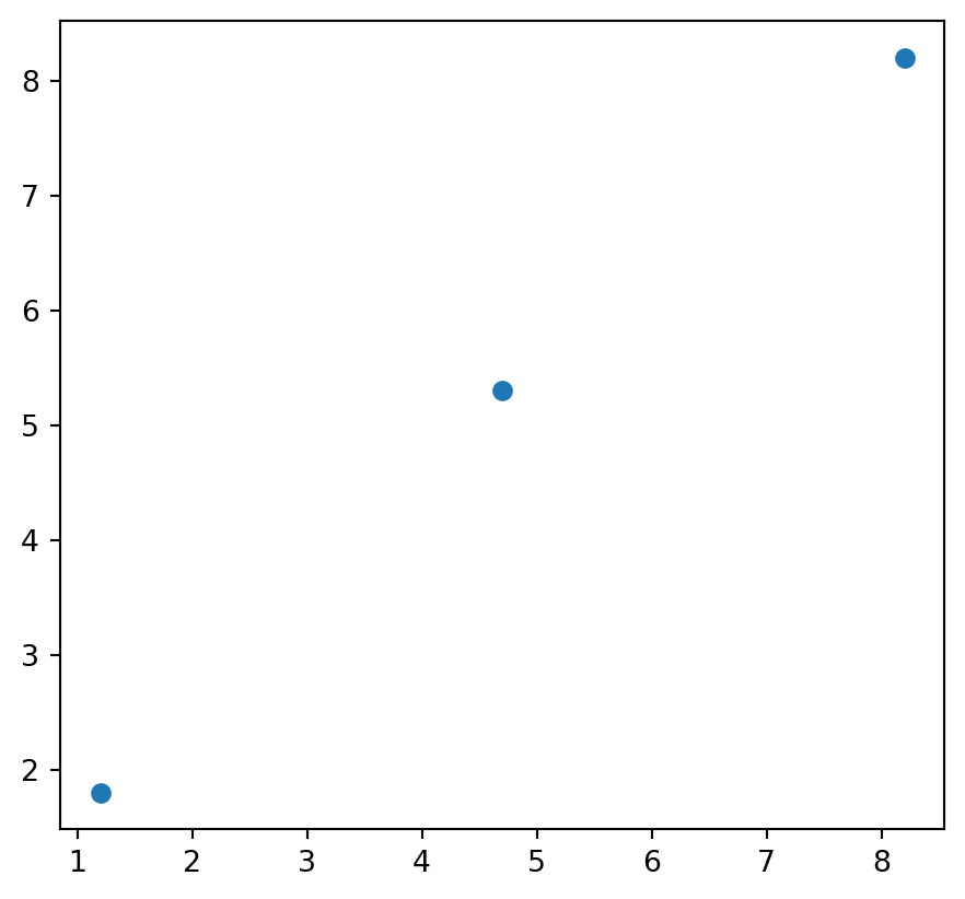
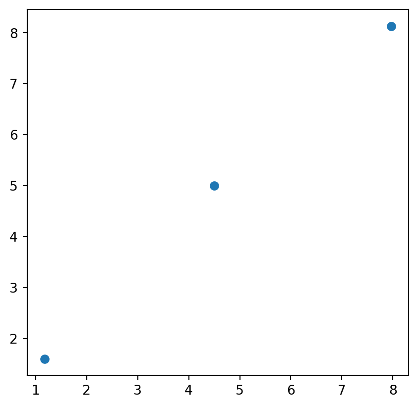
schools = gpd.GeoSeries(school_points)

schools.plot()

type(schools)

geopandas.geoseries.GeoSeries

GeoDataFrame

A GeoDataFrame is similar to a pandas DataFrame but includes at least one GeoSeries and supports spatial operations on its data.

schools_gdf = gpd.GeoDataFrame(geometry=schools)

schools_gdf.head()

	geometry
0	POINT (1.2 1.8)
1	POINT (4.7 5.3)
2	POINT (8.2 8.2)

type(schools_gdf)

geopandas.geodataframe.GeoDataFrame

schools_gdf['students'] = [124, 94, 100]

schools_gdf.head()

	geometry	students
0	POINT (1.2 1.8)	124
1	POINT (4.7 5.3)	94
2	POINT (8.2 8.2)	100

schools_gdf.plot()

schools_gdf.plot(column='students')

streets_gdf = gpd.GeoDataFrame(geometry=streets)

streets_gdf.plot()

streets_gdf['length'] = streets_gdf.length

streets_gdf.head()

	geometry	length
0	LINESTRING (0 0, 1 2, 3 3)	4.472136
1	LINESTRING (3 3, 5 2, 7 5)	5.841619
2	LINESTRING (7 5, 8 8, 10 10)	5.990705
3	LINESTRING (1 2, 2 5, 4 6)	5.398346

streets_gdf.plot(column='length', legend=True)

catchments_gdf = gpd.GeoDataFrame(geometry=catchment_polygons)

catchments_gdf['area'] = catchments_gdf.area
catchments_gdf.plot(column='area', legend=True)

The `geometry` of a GeoDataFrame

One of the key differences between a GeoDataFrame and a pandas DataFrame is that the former will have a geometry column that holds a GeoSeries:

catchments_gdf.geometry

0    POLYGON ((0.5 0.5, 2 1, 1.5 3, 0.5 2, 0.5 0.5))
1            POLYGON ((3 4, 5 3.5, 6 6, 4 6.5, 3 4))
2          POLYGON ((7 7, 8.5 7.5, 9 9, 7.5 9, 7 7))
Name: geometry, dtype: geometry

catchments_gdf.head()

	geometry	area
0	POLYGON ((0.5 0.5, 2 1, 1.5 3, 0.5 2, 0.5 0.5))	2.375
1	POLYGON ((3 4, 5 3.5, 6 6, 4 6.5, 3 4))	5.500
2	POLYGON ((7 7, 8.5 7.5, 9 9, 7.5 9, 7 7))	2.500

A GeoDataFrame can contained more than a single GeoSeries but only one can be operative as far as the geometry attribute is concerned. To see this, let’s add a second GeoSeries to the catchments GeoDataFrame:

catchments_gdf.centroid

0    POINT (1.17544 1.60526)
1              POINT (4.5 5)
2    POINT (7.96667 8.13333)
dtype: geometry

catchments_gdf['centroid_point'] = catchments_gdf.centroid
catchments_gdf.head()

	geometry	area	centroid_point
0	POLYGON ((0.5 0.5, 2 1, 1.5 3, 0.5 2, 0.5 0.5))	2.375	POINT (1.17544 1.60526)
1	POLYGON ((3 4, 5 3.5, 6 6, 4 6.5, 3 4))	5.500	POINT (4.5 5)
2	POLYGON ((7 7, 8.5 7.5, 9 9, 7.5 9, 7 7))	2.500	POINT (7.96667 8.13333)

Now we can set the geometry to be the centroid_point GeoSeries:

catchments_gdf.set_geometry('centroid_point', inplace=True)
catchments_gdf.plot()

And we could return to the polygons with:

catchments_gdf.set_geometry('geometry', inplace=True)
catchments_gdf.plot()

--- title: GeoPandas format: html: code-fold: false jupyter: python3 execute: cache: true --- ## Geometries for Vector Spatial Data Earlier in the course we had a figure to illustrate vector spatial data: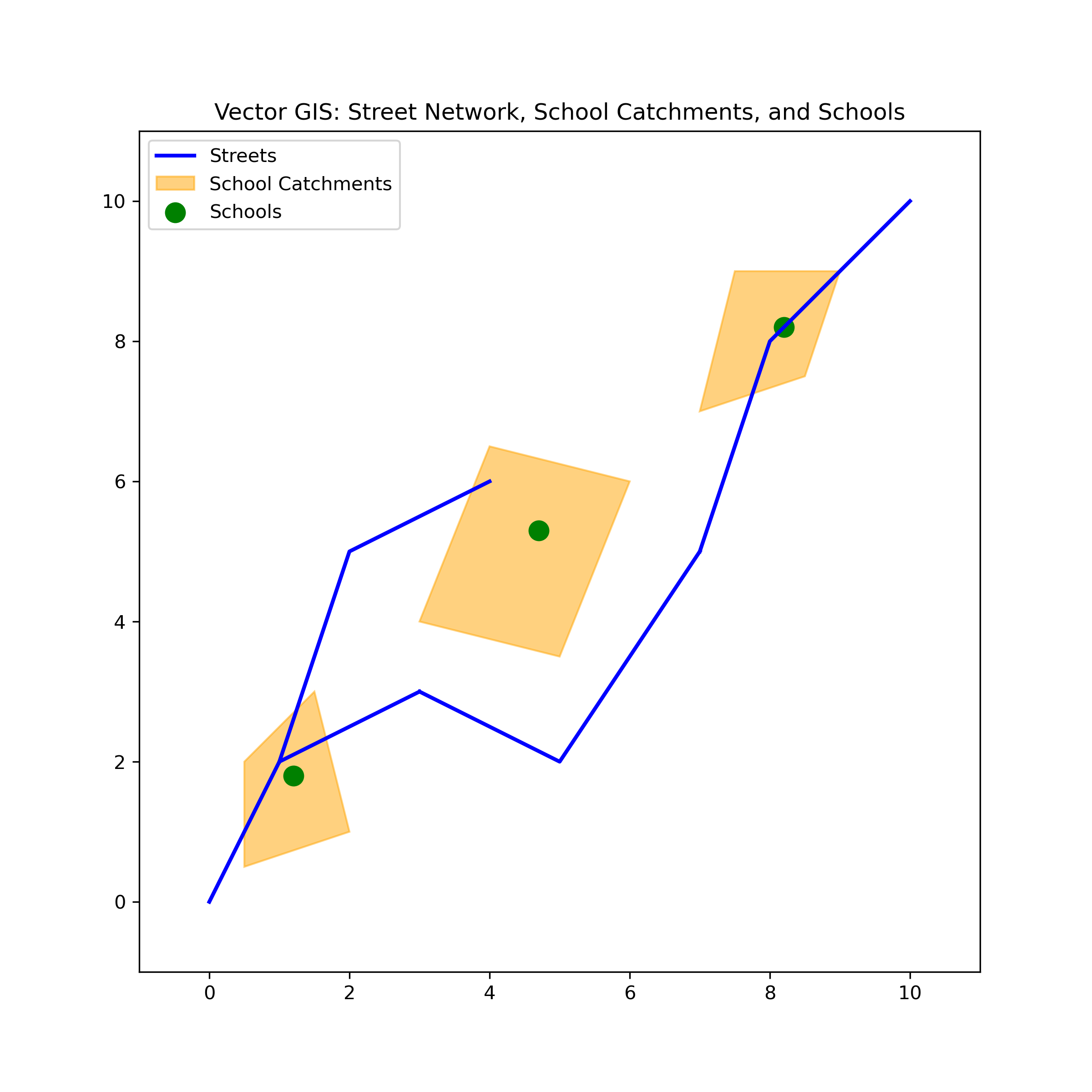 ![Vector GIS](vector.png) This figure was built with the following code: ```{python} import matplotlib.pyplot as plt from matplotlib.patches import Polygon as MplPolygon # Data for streets (line strings) streets = [ [(0, 0), (1, 2), (3, 3)], [(3, 3), (5, 2), (7, 5)], [(7, 5), (8, 8), (10, 10)], [(1, 2), (2, 5), (4, 6)], ] # Data for school catchments (polygons) catchments = [ [(0.5, 0.5), (2, 1), (1.5, 3), (0.5, 2)], [(3, 4), (5, 3.5), (6, 6), (4, 6.5)], [(7, 7), (8.5, 7.5), (9, 9), (7.5, 9)], ] # Adjusting the data for one school per catchment schools = [(1.2, 1.8), (4.7, 5.3), (8.2, 8.2)] # Plotting the GIS map with one school per catchment fig, ax = plt.subplots(figsize=(8, 8)) # Plotting the streets with one legend entry ax.plot(*zip(*streets[0]), color='blue', linewidth=2, label="Streets") for street in streets[1:]: street_x, street_y = zip(*street) ax.plot(street_x, street_y, color='blue', linewidth=2) # Plotting the catchments with legend for i, catchment in enumerate(catchments): polygon = MplPolygon(catchment, closed=True, color='orange', alpha=0.5, edgecolor='black') ax.add_patch(polygon) if i == 0: polygon.set_label("School Catchments") # Plotting the schools (points) with one per catchment school_x, school_y = zip(*schools) ax.scatter(school_x, school_y, color='green', s=100, label="Schools") # Set the legend and title ax.legend() ax.set_title('Vector GIS: Street Network, School Catchments, and Schools') ax.set_xlim(-1, 11) ax.set_ylim(-1, 11) ax.set_aspect('equal') # Save the figure to a file plt.savefig("vector.png", dpi=300) # Show the plot plt.show() ``` Here, we are faking it regarding a GIS, as matplotlib is a visualization library and doesn't actually allow us to do any spatial analysis per se. Fortunately, there are a number of Python packages that are designed to wrangle spatial data: - shapely - GeoPandas ## shapely [Shapely](https://shapely.readthedocs.io/en/stable/manual.html) [@shapely2007] is a Python package for the manipulation and analysis of [planar]( https://www.merriam-webster.com/dictionary/planar) geometric objects. We can use shapely to build up our example, starting with its `Point` class: ```{python} from shapely import Point ``` The `Point` class can be used to create instances for each of our schools, here using a python [list comprehension](https://www.w3schools.com/Python/python_lists_comprehension.asp): ```{python} school_points = [Point(school) for school in schools] ``` This results in a python list containing three shapely point objects: ```{python} school_points ``` If we ask for the first point, we get a rendered point. ```{python} school_points[0] ``` And, if we unpack the list into individual points, we should see similar behavior. ```{python} school_0, school_1, school_2 = school_points ``` ```{python} school_0 ``` ```{python} school_1 ``` ```{python} school_2 ``` Just like we did for points, we can rely on shapely for dealing with our catchments, but this time using the `Polygon` class: ```{python} from shapely import Polygon ``` ```{python} catchment_polygons = [Polygon(catchment) for catchment in catchments] ``` ```{python} catchment_0, catchment_1, catchment_2 = catchment_polygons ``` ```{python} catchment_0 ``` ```{python} catchment_1 ``` ```{python} catchment_2 ``` And, finally, we can model the road network using the `LineString` class: ```{python} from shapely import LineString ``` ```{python} street_lines = [LineString(street) for street in streets] ``` ```{python} street_0, street_1, street_2, street_3 = street_lines ``` ```{python} street_0 ``` ```{python} street_1 ``` ```{python} street_2 ``` ```{python} street_3 ``` ### shapely Geometry Types ```{python} school_0.geom_type ``` ```{python} school_2.geom_type ``` Points are zero-dimensional geometries, and thus have 0 area and 0 length: ```{python} school_0.area ``` ```{python} school_0.length ``` ```{python} list(school_0.coords) ``` ```{python} list(school_2.coords) ``` LineStrings are one-dimensional geometric objects, having length but 0 area ```{python} street_1.length ``` ```{python} street_1.area ``` Finally, Polygons are two-dimensional geometric objects, having area: ```{python} catchment_1.area ``` as well as length: ```{python} catchment_1.length ``` ### geometry methods and spatial predicates The power of these geometries comes from the functions and abilities to evaluate [spatial predicates](https://shapely.readthedocs.io/en/stable/predicates.html). These give us the building blocks of GIS operations for vector spatial data: To see this, we can call the `distance` method of `school_0` to determine the distance separating it from `school_2`: ```{python} school_0.distance(school_2) ``` We can also measure the difference between objects of different geometry types: ```{python} street_1.geom_type ``` ```{python} school_0.distance(street_1) ``` ```{python} catchment_0.geom_type ``` ```{python} catchment_0.area ``` ```{python} list(catchment_0.exterior.coords) ``` ```{python} catchment_0.bounds ``` ```{python} school_0.distance(catchment_0) ``` ```{python} catchment_0.contains(school_0) ``` ```{python} catchment_0.contains(school_1) ``` ```{python} school_1.distance(catchment_0) ``` ::: {.callout-note} All the area, distance, and other measurements done with shapely objects utilize [Cartesian coordinates](https://shapely.readthedocs.io/en/stable/manual.html#coordinate-systems). ::: ## GeoPandas [GeoPandas](https://geopandas.org/en/stable/) [@kelsey_jordahl_2020_3946761] is a python package that makes working with geospatial data easier. It relies on shapely and other libraries to extend the datatypes used by Pandas to allow spatial operations on geometric types. The two important classes in GeoPandas are: - `GeoSeries` - `GeoDataFrame` These are spatial extensions of the `Series` and `DataFrame` classes from `pandas`. ### import and aliasing ```{python} import geopandas as gpd ``` ### GeoSeries A [`GeoSeries`](https://geopandas.org/en/stable/docs/reference/geoseries.html) is essentially a `pandas` `Series` object designed to store `shapely` geometry types: ```{python} streets = gpd.GeoSeries(street_lines) ``` ```{python} streets.plot() ``` ```{python} catchments = gpd.GeoSeries(catchment_polygons) ``` ```{python} catchments.plot() ``` ```{python} schools = gpd.GeoSeries(school_points) ``` ```{python} schools.plot() ``` ```{python} type(schools) ``` ### GeoDataFrame A [`GeoDataFrame`](https://geopandas.org/en/stable/docs/reference/geodataframe.html) is similar to a pandas DataFrame but includes at least one `GeoSeries` and supports spatial operations on its data. ```{python} schools_gdf = gpd.GeoDataFrame(geometry=schools) ``` ```{python} schools_gdf.head() ``` ```{python} type(schools_gdf) ``` ```{python} schools_gdf['students'] = [124, 94, 100] ``` ```{python} schools_gdf.head() ``` ```{python} schools_gdf.plot() ``` ```{python} schools_gdf.plot(column='students') ``` ```{python} streets_gdf = gpd.GeoDataFrame(geometry=streets) ``` ```{python} streets_gdf.plot() ``` ```{python} streets_gdf['length'] = streets_gdf.length ``` ```{python} streets_gdf.head() ``` ```{python} streets_gdf.plot(column='length', legend=True) ``` ```{python} catchments_gdf = gpd.GeoDataFrame(geometry=catchment_polygons) ``` ```{python} catchments_gdf['area'] = catchments_gdf.area catchments_gdf.plot(column='area', legend=True) ``` ### The `geometry` of a GeoDataFrame One of the key differences between a `GeoDataFrame` and a pandas `DataFrame` is that the former will have a `geometry` column that holds a `GeoSeries`: ```{python} catchments_gdf.geometry ``` ```{python} catchments_gdf.head() ``` A `GeoDataFrame` can contained more than a single `GeoSeries` but only one can be operative as far as the `geometry` attribute is concerned. To see this, let's add a second `GeoSeries` to the catchments `GeoDataFrame`: ```{python} catchments_gdf.centroid ``` ```{python} catchments_gdf['centroid_point'] = catchments_gdf.centroid catchments_gdf.head() ``` Now we can set the geometry to be the `centroid_point` `GeoSeries`: ```{python} catchments_gdf.set_geometry('centroid_point', inplace=True) catchments_gdf.plot() ``` And we could return to the polygons with: ```{python} catchments_gdf.set_geometry('geometry', inplace=True) catchments_gdf.plot() ```

Geometries for Vector Spatial Data

shapely

shapely Geometry Types

geometry methods and spatial predicates

GeoPandas

import and aliasing

GeoSeries

GeoDataFrame

The geometry of a GeoDataFrame

The `geometry` of a GeoDataFrame