Introduction to Pandas

Author

Serge Rey

Introduction

In this notebook we introduce pandas (mckinney-proc-scipy-2010?) which is the main package for working with data in Python.

Import

We start by importing the package, and aliasing it as pd

import pandas as pd

Aliasing allows us to use pd in place of having to type out pandas in what follows.

DataFrame Creation

Pandas main data structure is called a DataFrame. We will create our first DataFrame by reading a csv file.

1home = "/home/serge"
cities_df = pd.read_csv(f"{home}/data/385/studio02/cities.csv")

1: Change the value home to be equal to jupyter-student where student is your id.

Warning

Be sure to reread the instructions to change the path in the previous cell if you wish to follow along in your own notebook.

Asking for the values of the cities_df give us:

cities_df

	name	description	latitude	longitude
0	Alabama	Montgomery	32.377716	-86.300568
1	Alaska	Juneau	58.301598	-134.420212
2	Arizona	Phoenix	33.448143	-112.096962
3	Arkansas	Little Rock	34.746613	-92.288986
4	California	Sacramento	38.576668	-121.493629
5	Colorado	Denver	39.739227	-104.984856
6	Connecticut	Hartford<br>	41.764046	-72.682198
7	Delaware	Dover	39.157307	-75.519722
8	Hawaii	Honolulu	21.307442	-157.857376
9	Florida	Tallahassee	30.438118	-84.281296
10	Georgia	Atlanta<br>	33.749027	-84.388229
11	Idaho	Boise	43.617775	-116.199722
12	Illinois	Springfield	39.798363	-89.654961
13	Indiana	Indianapolis	39.768623	-86.162643
14	Iowa	Des Moines	41.591087	-93.603729
15	Kansas	Topeka	39.048191	-95.677956
16	Kentucky	Frankfort	38.186722	-84.875374
17	Louisiana	Baton Rouge	30.457069	-91.187393
18	Maine	Augusta	44.307167	-69.781693
19	Maryland	Annapolis	38.978764	-76.490936
20	Massachusetts	Boston	42.358162	-71.063698
21	Michigan	Lansing	42.733635	-84.555328
22	Minnesota	St. Paul	44.955097	-93.102211
23	Mississippi	Jackson	32.303848	-90.182106
24	Missouri	Jefferson City	38.579201	-92.172935
25	Montana	Helena	46.585709	-112.018417
26	Nebraska	Lincoln	40.808075	-96.699654
27	Nevada	Carson City	39.163914	-119.766121
28	New Hampshire	Concord	43.206898	-71.537994
29	New Jersey	Trenton	40.220596	-74.769913
30	New Mexico	Santa Fe	35.682240	-105.939728
31	North Carolina	Raleigh	35.780430	-78.639099
32	North Dakota	Bismarck	46.820850	-100.783318
33	New York	Albany	42.652843	-73.757874
34	Ohio	Columbus	39.961346	-82.999069
35	Oklahoma	Oklahoma City	35.492207	-97.503342
36	Oregon	Salem	44.938461	-123.030403
37	Pennsylvania	Harrisburg	40.264378	-76.883598
38	Rhode Island	Providence	41.830914	-71.414963
39	South Carolina	Columbia	34.000343	-81.033211
40	South Dakota	Pierre	44.367031	-100.346405
41	Tennessee	Nashville	36.165810	-86.784241
42	Texas	Austin	30.274670	-97.740349
43	Utah	Salt Lake City	40.777477	-111.888237
44	Vermont	Montpelier	44.262436	-72.580536
45	Virginia	Richmond	37.538857	-77.433640
46	Washington	Olympia	47.035805	-122.905014
47	West Virginia	Charleston	38.336246	-81.612328
48	Wisconsin	Madison	43.074684	-89.384445
49	Wyoming	Cheyenne	41.140259	-104.820236

This data set is composed of the capital cities for the 50 states.

We can see what type of object cities_df is using type:

type(cities_df)

pandas.core.frame.DataFrame

As an analogy, you can think of a DataFrame as a spreadsheet with rows and columns. This mental model will help to orient you. We will see that the DataFrame extends spreadsheets in powerful ways for data analysis.

A DataFrame, like most Python objects, has a number of attributes and methods.

Its shape attribute tells us how many observations and variables we have.

cities_df.shape

(50, 4)

In this case our data set has 50 observations on 4 variables.

Series

Each variable is stored as a Series:

type(cities_df.longitude)

pandas.core.series.Series

cities_df.longitude

0     -86.300568
1    -134.420212
2    -112.096962
3     -92.288986
4    -121.493629
5    -104.984856
6     -72.682198
7     -75.519722
8    -157.857376
9     -84.281296
10    -84.388229
11   -116.199722
12    -89.654961
13    -86.162643
14    -93.603729
15    -95.677956
16    -84.875374
17    -91.187393
18    -69.781693
19    -76.490936
20    -71.063698
21    -84.555328
22    -93.102211
23    -90.182106
24    -92.172935
25   -112.018417
26    -96.699654
27   -119.766121
28    -71.537994
29    -74.769913
30   -105.939728
31    -78.639099
32   -100.783318
33    -73.757874
34    -82.999069
35    -97.503342
36   -123.030403
37    -76.883598
38    -71.414963
39    -81.033211
40   -100.346405
41    -86.784241
42    -97.740349
43   -111.888237
44    -72.580536
45    -77.433640
46   -122.905014
47    -81.612328
48    -89.384445
49   -104.820236
Name: longitude, dtype: float64

When we ask for the contents of the series, we see two columns of numbers. The first is a set of integers which is the index. Each value in the index locates the particular observation in the series.

The next column of values stores the values of the series. Here the values are decimal degrees of longitude for the capital cities.

Data Types

The info method of the DataFrame will summarize information about our DataFrame

cities_df.info()

<class 'pandas.core.frame.DataFrame'>
RangeIndex: 50 entries, 0 to 49
Data columns (total 4 columns):
 #   Column       Non-Null Count  Dtype  
---  ------       --------------  -----  
 0   name         50 non-null     object 
 1   description  50 non-null     object 
 2   latitude     50 non-null     float64
 3   longitude    50 non-null     float64
dtypes: float64(2), object(2)
memory usage: 1.7+ KB

We have four columns, the first two of which are of type object and the last two are of type float64.

The names of our variables in the DataFrame are stored in the columns attribute:

cities_df.columns

Index(['name', 'description', 'latitude', 'longitude'], dtype='object')

We can use the column name to access the particular series:

cities_df.longitude

0     -86.300568
1    -134.420212
2    -112.096962
3     -92.288986
4    -121.493629
5    -104.984856
6     -72.682198
7     -75.519722
8    -157.857376
9     -84.281296
10    -84.388229
11   -116.199722
12    -89.654961
13    -86.162643
14    -93.603729
15    -95.677956
16    -84.875374
17    -91.187393
18    -69.781693
19    -76.490936
20    -71.063698
21    -84.555328
22    -93.102211
23    -90.182106
24    -92.172935
25   -112.018417
26    -96.699654
27   -119.766121
28    -71.537994
29    -74.769913
30   -105.939728
31    -78.639099
32   -100.783318
33    -73.757874
34    -82.999069
35    -97.503342
36   -123.030403
37    -76.883598
38    -71.414963
39    -81.033211
40   -100.346405
41    -86.784241
42    -97.740349
43   -111.888237
44    -72.580536
45    -77.433640
46   -122.905014
47    -81.612328
48    -89.384445
49   -104.820236
Name: longitude, dtype: float64

cities_df.name

0            Alabama
1             Alaska
2            Arizona
3           Arkansas
4         California
5           Colorado
6        Connecticut
7           Delaware
8             Hawaii
9            Florida
10           Georgia
11             Idaho
12          Illinois
13           Indiana
14              Iowa
15            Kansas
16          Kentucky
17         Louisiana
18             Maine
19          Maryland
20     Massachusetts
21          Michigan
22         Minnesota
23       Mississippi
24          Missouri
25           Montana
26          Nebraska
27            Nevada
28     New Hampshire
29        New Jersey
30        New Mexico
31    North Carolina
32      North Dakota
33          New York
34              Ohio
35          Oklahoma
36            Oregon
37      Pennsylvania
38      Rhode Island
39    South Carolina
40      South Dakota
41         Tennessee
42             Texas
43              Utah
44           Vermont
45          Virginia
46        Washington
47     West Virginia
48         Wisconsin
49           Wyoming
Name: name, dtype: object

As each series is an object, it too comes with attributes and methods:

cities_df.longitude.max()

np.float64(-69.781693)

cities_df.name.max()

'Wyoming'

cities_df.longitude.mean()

np.float64(-93.46593707999999)

cities_df.name.min()

'Alabama'

cities_df.longitude.describe()

count     50.000000
mean     -93.465937
std       18.669710
min     -157.857376
25%     -103.811006
50%      -89.918533
75%      -79.237627
max      -69.781693
Name: longitude, dtype: float64

cities_df.name.describe()

count          50
unique         50
top       Alabama
freq            1
Name: name, dtype: object

Note how the same method behaves for series of different types.

Creating new series

A common workflow in data analysis is to create, or derive, new variables based upon existing variables. For example, let’s define a variable that will denote whether a capital city is in the east or west of the country. Here we will use the median longitude as the comparison point:

cities_df.longitude.median()

np.float64(-89.9185335)

cities_df.longitude < cities_df.longitude.median()

0     False
1      True
2      True
3      True
4      True
5      True
6     False
7     False
8      True
9     False
10    False
11     True
12    False
13    False
14     True
15     True
16    False
17     True
18    False
19    False
20    False
21    False
22     True
23     True
24     True
25     True
26     True
27     True
28    False
29    False
30     True
31    False
32     True
33    False
34    False
35     True
36     True
37    False
38    False
39    False
40     True
41    False
42     True
43     True
44    False
45    False
46     True
47    False
48    False
49     True
Name: longitude, dtype: bool

This creates a series that has data type bool, meaning True if the city is at a longitude less than that of the median longitude. False if it is east of that value. We can use this information to create a new series on the DataFrame called east:

cities_df['east'] = cities_df.longitude > cities_df.longitude.median()

And, we can do this for a second variable south:

cities_df['south'] = cities_df.latitude < cities_df.latitude.median()

Based on those two Boolean variables we can create an additional variable called region that tells us which of four regions the capital city is located in.

cities_df['region'] = 4 * cities_df.east * cities_df.south + 3 * (1 - cities_df.east) * cities_df.south \
                      + 2 * (1-cities_df.east) * (1-cities_df.south) + cities_df.east * (1-cities_df.south)

region takes on four values, 1 if the city is in the North East, 2 North West, 3 South West, and 4 South East.

cities_df.head(20)

	name	description	latitude	longitude	east	south	region
0	Alabama	Montgomery	32.377716	-86.300568	True	True	4
1	Alaska	Juneau	58.301598	-134.420212	False	False	2
2	Arizona	Phoenix	33.448143	-112.096962	False	True	3
3	Arkansas	Little Rock	34.746613	-92.288986	False	True	3
4	California	Sacramento	38.576668	-121.493629	False	True	3
5	Colorado	Denver	39.739227	-104.984856	False	True	3
6	Connecticut	Hartford<br>	41.764046	-72.682198	True	False	1
7	Delaware	Dover	39.157307	-75.519722	True	True	4
8	Hawaii	Honolulu	21.307442	-157.857376	False	True	3
9	Florida	Tallahassee	30.438118	-84.281296	True	True	4
10	Georgia	Atlanta<br>	33.749027	-84.388229	True	True	4
11	Idaho	Boise	43.617775	-116.199722	False	False	2
12	Illinois	Springfield	39.798363	-89.654961	True	False	1
13	Indiana	Indianapolis	39.768623	-86.162643	True	True	4
14	Iowa	Des Moines	41.591087	-93.603729	False	False	2
15	Kansas	Topeka	39.048191	-95.677956	False	True	3
16	Kentucky	Frankfort	38.186722	-84.875374	True	True	4
17	Louisiana	Baton Rouge	30.457069	-91.187393	False	True	3
18	Maine	Augusta	44.307167	-69.781693	True	False	1
19	Maryland	Annapolis	38.978764	-76.490936	True	True	4

Plotting

Pandas comes with built-in plotting facilities. We can try out the default plot method:

cities_df.plot('longitude', 'latitude')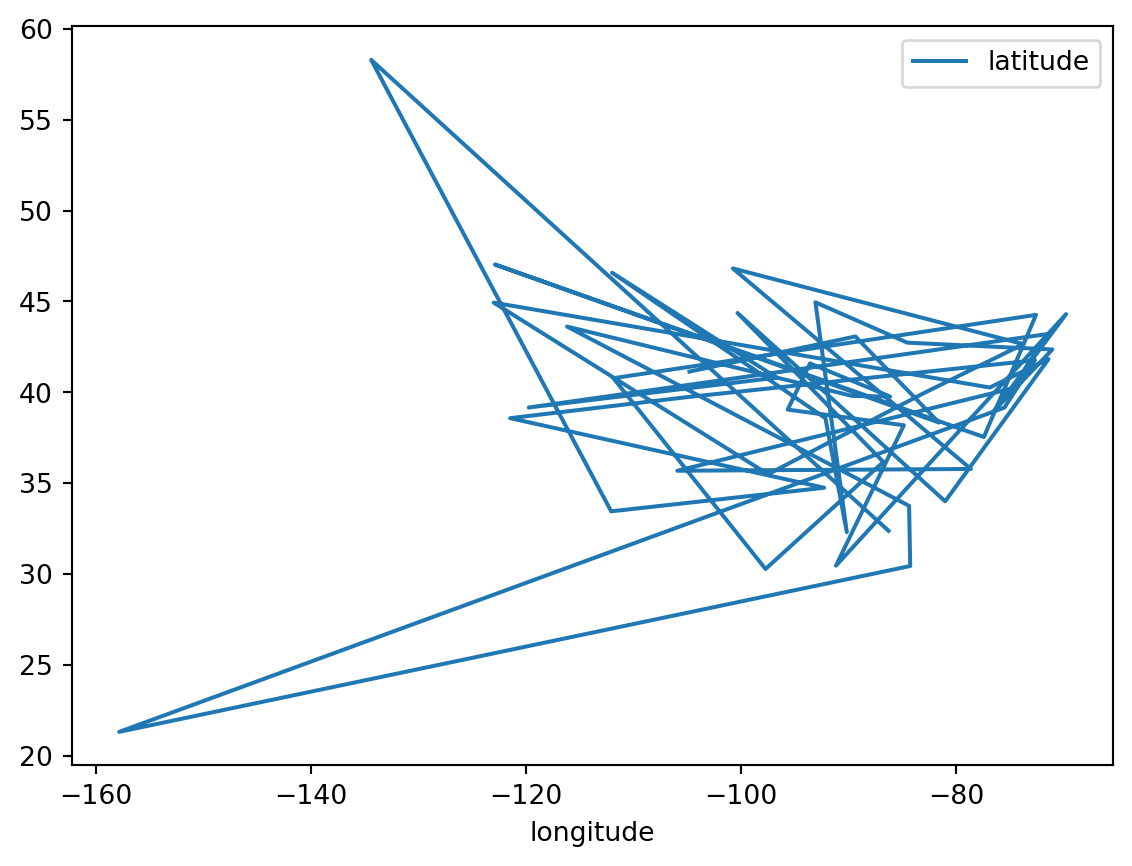

This isn’t quite what we want as the default is to plot the first series and the second series together with line segments connecting each pair of sequential observations.

But we can try a different method to get what we want:

cities_df.plot.scatter('longitude', 'latitude')

That’s better as now we see the cities represented as points.

Warning

We are treating longitude and latitude as Cartesian coordinates in the plots. This is technically not correct as they are spherical coordinates. We will correct this later on in the course when we get to spatial data analysis proper.

There are a number of powerful visualization packages in Python that allow us to go beyond what is available in Pandas. To see one of them here, we import seaborn

import seaborn as sbn

and redo our plot:

sbn.scatterplot(cities_df, x='longitude', y='latitude');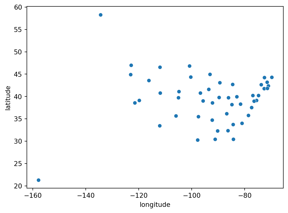

So far, not much difference from what we did with pandas. But we can specify a hue variable to distinguish what region the cities are in:

sbn.scatterplot(cities_df, x='longitude', y='latitude', hue='region');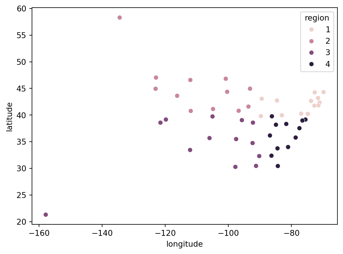

Great. But the numbers on the legend are not that informative. Let’s change them:

cities_df.region.map({1:'NE', 2:'NW', 3:'SW', 4:'SE'})

0     SE
1     NW
2     SW
3     SW
4     SW
5     SW
6     NE
7     SE
8     SW
9     SE
10    SE
11    NW
12    NE
13    SE
14    NW
15    SW
16    SE
17    SW
18    NE
19    SE
20    NE
21    NE
22    NW
23    SW
24    SW
25    NW
26    NW
27    SW
28    NE
29    NE
30    SW
31    SE
32    NW
33    NE
34    NE
35    SW
36    NW
37    NE
38    NE
39    SE
40    NW
41    SE
42    SW
43    NW
44    NE
45    SE
46    NW
47    SE
48    NE
49    NW
Name: region, dtype: object

cities_df['region'] = cities_df.region.map({1:'NE', 2:'NW', 3:'SW', 4:'SE'})

sbn.scatterplot(cities_df, x='longitude', y='latitude', hue='region');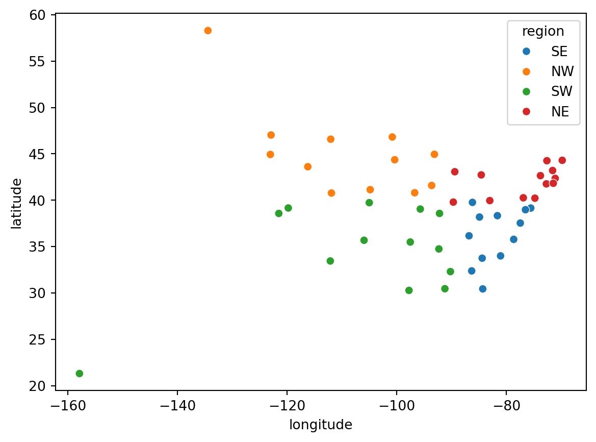

Much better.

cities_df.head()

	name	description	latitude	longitude	east	south	region
0	Alabama	Montgomery	32.377716	-86.300568	True	True	SE
1	Alaska	Juneau	58.301598	-134.420212	False	False	NW
2	Arizona	Phoenix	33.448143	-112.096962	False	True	SW
3	Arkansas	Little Rock	34.746613	-92.288986	False	True	SW
4	California	Sacramento	38.576668	-121.493629	False	True	SW

DataFrame Operations

Pandas has a number of powerful methods that allow us to manipulate the DataFrame in interesting ways. Here we look at three:

sorting
grouping
filtering

Sorting

We can sort the DataFrame by the values of a given column. For example, to find the southern-most capital city:

cities_df.sort_values(by='latitude')

	name	description	latitude	longitude	east	south	region
8	Hawaii	Honolulu	21.307442	-157.857376	False	True	SW
42	Texas	Austin	30.274670	-97.740349	False	True	SW
9	Florida	Tallahassee	30.438118	-84.281296	True	True	SE
17	Louisiana	Baton Rouge	30.457069	-91.187393	False	True	SW
23	Mississippi	Jackson	32.303848	-90.182106	False	True	SW
0	Alabama	Montgomery	32.377716	-86.300568	True	True	SE
2	Arizona	Phoenix	33.448143	-112.096962	False	True	SW
10	Georgia	Atlanta<br>	33.749027	-84.388229	True	True	SE
39	South Carolina	Columbia	34.000343	-81.033211	True	True	SE
3	Arkansas	Little Rock	34.746613	-92.288986	False	True	SW
35	Oklahoma	Oklahoma City	35.492207	-97.503342	False	True	SW
30	New Mexico	Santa Fe	35.682240	-105.939728	False	True	SW
31	North Carolina	Raleigh	35.780430	-78.639099	True	True	SE
41	Tennessee	Nashville	36.165810	-86.784241	True	True	SE
45	Virginia	Richmond	37.538857	-77.433640	True	True	SE
16	Kentucky	Frankfort	38.186722	-84.875374	True	True	SE
47	West Virginia	Charleston	38.336246	-81.612328	True	True	SE
4	California	Sacramento	38.576668	-121.493629	False	True	SW
24	Missouri	Jefferson City	38.579201	-92.172935	False	True	SW
19	Maryland	Annapolis	38.978764	-76.490936	True	True	SE
15	Kansas	Topeka	39.048191	-95.677956	False	True	SW
7	Delaware	Dover	39.157307	-75.519722	True	True	SE
27	Nevada	Carson City	39.163914	-119.766121	False	True	SW
5	Colorado	Denver	39.739227	-104.984856	False	True	SW
13	Indiana	Indianapolis	39.768623	-86.162643	True	True	SE
12	Illinois	Springfield	39.798363	-89.654961	True	False	NE
34	Ohio	Columbus	39.961346	-82.999069	True	False	NE
29	New Jersey	Trenton	40.220596	-74.769913	True	False	NE
37	Pennsylvania	Harrisburg	40.264378	-76.883598	True	False	NE
43	Utah	Salt Lake City	40.777477	-111.888237	False	False	NW
26	Nebraska	Lincoln	40.808075	-96.699654	False	False	NW
49	Wyoming	Cheyenne	41.140259	-104.820236	False	False	NW
14	Iowa	Des Moines	41.591087	-93.603729	False	False	NW
6	Connecticut	Hartford<br>	41.764046	-72.682198	True	False	NE
38	Rhode Island	Providence	41.830914	-71.414963	True	False	NE
20	Massachusetts	Boston	42.358162	-71.063698	True	False	NE
33	New York	Albany	42.652843	-73.757874	True	False	NE
21	Michigan	Lansing	42.733635	-84.555328	True	False	NE
48	Wisconsin	Madison	43.074684	-89.384445	True	False	NE
28	New Hampshire	Concord	43.206898	-71.537994	True	False	NE
11	Idaho	Boise	43.617775	-116.199722	False	False	NW
44	Vermont	Montpelier	44.262436	-72.580536	True	False	NE
18	Maine	Augusta	44.307167	-69.781693	True	False	NE
40	South Dakota	Pierre	44.367031	-100.346405	False	False	NW
36	Oregon	Salem	44.938461	-123.030403	False	False	NW
22	Minnesota	St. Paul	44.955097	-93.102211	False	False	NW
25	Montana	Helena	46.585709	-112.018417	False	False	NW
32	North Dakota	Bismarck	46.820850	-100.783318	False	False	NW
46	Washington	Olympia	47.035805	-122.905014	False	False	NW
1	Alaska	Juneau	58.301598	-134.420212	False	False	NW

To find the northern-most city:

cities_df.sort_values(by='latitude', ascending=False)

	name	description	latitude	longitude	east	south	region
1	Alaska	Juneau	58.301598	-134.420212	False	False	NW
46	Washington	Olympia	47.035805	-122.905014	False	False	NW
32	North Dakota	Bismarck	46.820850	-100.783318	False	False	NW
25	Montana	Helena	46.585709	-112.018417	False	False	NW
22	Minnesota	St. Paul	44.955097	-93.102211	False	False	NW
36	Oregon	Salem	44.938461	-123.030403	False	False	NW
40	South Dakota	Pierre	44.367031	-100.346405	False	False	NW
18	Maine	Augusta	44.307167	-69.781693	True	False	NE
44	Vermont	Montpelier	44.262436	-72.580536	True	False	NE
11	Idaho	Boise	43.617775	-116.199722	False	False	NW
28	New Hampshire	Concord	43.206898	-71.537994	True	False	NE
48	Wisconsin	Madison	43.074684	-89.384445	True	False	NE
21	Michigan	Lansing	42.733635	-84.555328	True	False	NE
33	New York	Albany	42.652843	-73.757874	True	False	NE
20	Massachusetts	Boston	42.358162	-71.063698	True	False	NE
38	Rhode Island	Providence	41.830914	-71.414963	True	False	NE
6	Connecticut	Hartford<br>	41.764046	-72.682198	True	False	NE
14	Iowa	Des Moines	41.591087	-93.603729	False	False	NW
49	Wyoming	Cheyenne	41.140259	-104.820236	False	False	NW
26	Nebraska	Lincoln	40.808075	-96.699654	False	False	NW
43	Utah	Salt Lake City	40.777477	-111.888237	False	False	NW
37	Pennsylvania	Harrisburg	40.264378	-76.883598	True	False	NE
29	New Jersey	Trenton	40.220596	-74.769913	True	False	NE
34	Ohio	Columbus	39.961346	-82.999069	True	False	NE
12	Illinois	Springfield	39.798363	-89.654961	True	False	NE
13	Indiana	Indianapolis	39.768623	-86.162643	True	True	SE
5	Colorado	Denver	39.739227	-104.984856	False	True	SW
27	Nevada	Carson City	39.163914	-119.766121	False	True	SW
7	Delaware	Dover	39.157307	-75.519722	True	True	SE
15	Kansas	Topeka	39.048191	-95.677956	False	True	SW
19	Maryland	Annapolis	38.978764	-76.490936	True	True	SE
24	Missouri	Jefferson City	38.579201	-92.172935	False	True	SW
4	California	Sacramento	38.576668	-121.493629	False	True	SW
47	West Virginia	Charleston	38.336246	-81.612328	True	True	SE
16	Kentucky	Frankfort	38.186722	-84.875374	True	True	SE
45	Virginia	Richmond	37.538857	-77.433640	True	True	SE
41	Tennessee	Nashville	36.165810	-86.784241	True	True	SE
31	North Carolina	Raleigh	35.780430	-78.639099	True	True	SE
30	New Mexico	Santa Fe	35.682240	-105.939728	False	True	SW
35	Oklahoma	Oklahoma City	35.492207	-97.503342	False	True	SW
3	Arkansas	Little Rock	34.746613	-92.288986	False	True	SW
39	South Carolina	Columbia	34.000343	-81.033211	True	True	SE
10	Georgia	Atlanta<br>	33.749027	-84.388229	True	True	SE
2	Arizona	Phoenix	33.448143	-112.096962	False	True	SW
0	Alabama	Montgomery	32.377716	-86.300568	True	True	SE
23	Mississippi	Jackson	32.303848	-90.182106	False	True	SW
17	Louisiana	Baton Rouge	30.457069	-91.187393	False	True	SW
9	Florida	Tallahassee	30.438118	-84.281296	True	True	SE
42	Texas	Austin	30.274670	-97.740349	False	True	SW
8	Hawaii	Honolulu	21.307442	-157.857376	False	True	SW

If we don’t want to see all the other columns, we can subset the dataframe first:

cities_df[['name', 'description', 'latitude']].sort_values(by='latitude', ascending=False)

	name	description	latitude
1	Alaska	Juneau	58.301598
46	Washington	Olympia	47.035805
32	North Dakota	Bismarck	46.820850
25	Montana	Helena	46.585709
22	Minnesota	St. Paul	44.955097
36	Oregon	Salem	44.938461
40	South Dakota	Pierre	44.367031
18	Maine	Augusta	44.307167
44	Vermont	Montpelier	44.262436
11	Idaho	Boise	43.617775
28	New Hampshire	Concord	43.206898
48	Wisconsin	Madison	43.074684
21	Michigan	Lansing	42.733635
33	New York	Albany	42.652843
20	Massachusetts	Boston	42.358162
38	Rhode Island	Providence	41.830914
6	Connecticut	Hartford<br>	41.764046
14	Iowa	Des Moines	41.591087
49	Wyoming	Cheyenne	41.140259
26	Nebraska	Lincoln	40.808075
43	Utah	Salt Lake City	40.777477
37	Pennsylvania	Harrisburg	40.264378
29	New Jersey	Trenton	40.220596
34	Ohio	Columbus	39.961346
12	Illinois	Springfield	39.798363
13	Indiana	Indianapolis	39.768623
5	Colorado	Denver	39.739227
27	Nevada	Carson City	39.163914
7	Delaware	Dover	39.157307
15	Kansas	Topeka	39.048191
19	Maryland	Annapolis	38.978764
24	Missouri	Jefferson City	38.579201
4	California	Sacramento	38.576668
47	West Virginia	Charleston	38.336246
16	Kentucky	Frankfort	38.186722
45	Virginia	Richmond	37.538857
41	Tennessee	Nashville	36.165810
31	North Carolina	Raleigh	35.780430
30	New Mexico	Santa Fe	35.682240
35	Oklahoma	Oklahoma City	35.492207
3	Arkansas	Little Rock	34.746613
39	South Carolina	Columbia	34.000343
10	Georgia	Atlanta<br>	33.749027
2	Arizona	Phoenix	33.448143
0	Alabama	Montgomery	32.377716
23	Mississippi	Jackson	32.303848
17	Louisiana	Baton Rouge	30.457069
9	Florida	Tallahassee	30.438118
42	Texas	Austin	30.274670
8	Hawaii	Honolulu	21.307442

Grouping

The groupby method of the DataFrame allows us to split the dataframe, apply a function, and combine the results. This allows us to group data in interesting ways.

Suppose we wanted to know how many cities were in the east and west?

cities_df.groupby(by='east').count()

	name	description	latitude	longitude	south	region
east
False	25	25	25	25	25	25
True	25	25	25	25	25	25

And for south and north:

cities_df.groupby(by='south').count()

	name	description	latitude	longitude	east	region
south
False	25	25	25	25	25	25
True	25	25	25	25	25	25

How about by region?

cities_df.groupby(by='region').count()

	name	description	latitude	longitude	east	south
region
NE	13	13	13	13	13	13
NW	12	12	12	12	12	12
SE	12	12	12	12	12	12
SW	13	13	13	13	13	13

Note

As we will see later in the course, there are different notions of a spatial median. This will unravel the mystery of why we have equal numbers of cities in the north and south, and east and west, but not in the four regions.

In addition to applying the count method on the groubby object, we could use other functions. For example, we may want to know the median coordinate values in each of the four regions:

cities_df[['region', 'longitude', 'latitude']].groupby(by='region').median()

	longitude	latitude
region
NE	-73.757874	42.358162
NW	-108.354236	44.652746
SE	-82.946812	36.852334
SW	-97.740349	35.492207

Filtering

Filtering allows us to subset the DataFrame based on some conditions. For example, what if we wanted to create a new DataFrame that only contained the southern capital cities:

south_df = cities_df[cities_df.south]

south_df.shape

(25, 7)

south_df.head()

	name	description	latitude	longitude	east	south	region
0	Alabama	Montgomery	32.377716	-86.300568	True	True	SE
2	Arizona	Phoenix	33.448143	-112.096962	False	True	SW
3	Arkansas	Little Rock	34.746613	-92.288986	False	True	SW
4	California	Sacramento	38.576668	-121.493629	False	True	SW
5	Colorado	Denver	39.739227	-104.984856	False	True	SW

And to get a DataFrame for the northern cities, we could use a complement filter:

north_df = cities_df[~cities_df.south]

The ~ operator can be thought of flipping the boolean condition.

north_df.head()

	name	description	latitude	longitude	east	south	region
1	Alaska	Juneau	58.301598	-134.420212	False	False	NW
6	Connecticut	Hartford<br>	41.764046	-72.682198	True	False	NE
11	Idaho	Boise	43.617775	-116.199722	False	False	NW
12	Illinois	Springfield	39.798363	-89.654961	True	False	NE
14	Iowa	Des Moines	41.591087	-93.603729	False	False	NW

We could combine these to get the DataFrame for cities in the North East region:

ne_df = cities_df[~cities_df.south & cities_df.east]

ne_df.head()

	name	description	latitude	longitude	east	south	region
6	Connecticut	Hartford<br>	41.764046	-72.682198	True	False	NE
12	Illinois	Springfield	39.798363	-89.654961	True	False	NE
18	Maine	Augusta	44.307167	-69.781693	True	False	NE
20	Massachusetts	Boston	42.358162	-71.063698	True	False	NE
21	Michigan	Lansing	42.733635	-84.555328	True	False	NE

Like most things we will want to do, there are typically multiple ways to accomplish this in Python. Here we can get a set of regional DataFrames in one shot:

dfs = {r:data for r, data in cities_df.groupby('region')}

dfs

{'NE':              name   description   latitude  longitude  east  south region
 6     Connecticut  Hartford<br>  41.764046 -72.682198  True  False     NE
 12       Illinois   Springfield  39.798363 -89.654961  True  False     NE
 18          Maine       Augusta  44.307167 -69.781693  True  False     NE
 20  Massachusetts        Boston  42.358162 -71.063698  True  False     NE
 21       Michigan       Lansing  42.733635 -84.555328  True  False     NE
 28  New Hampshire       Concord  43.206898 -71.537994  True  False     NE
 29     New Jersey       Trenton  40.220596 -74.769913  True  False     NE
 33       New York        Albany  42.652843 -73.757874  True  False     NE
 34           Ohio      Columbus  39.961346 -82.999069  True  False     NE
 37   Pennsylvania    Harrisburg  40.264378 -76.883598  True  False     NE
 38   Rhode Island    Providence  41.830914 -71.414963  True  False     NE
 44        Vermont    Montpelier  44.262436 -72.580536  True  False     NE
 48      Wisconsin       Madison  43.074684 -89.384445  True  False     NE,
 'NW':             name     description   latitude   longitude   east  south region
 1         Alaska          Juneau  58.301598 -134.420212  False  False     NW
 11         Idaho           Boise  43.617775 -116.199722  False  False     NW
 14          Iowa      Des Moines  41.591087  -93.603729  False  False     NW
 22     Minnesota        St. Paul  44.955097  -93.102211  False  False     NW
 25       Montana          Helena  46.585709 -112.018417  False  False     NW
 26      Nebraska         Lincoln  40.808075  -96.699654  False  False     NW
 32  North Dakota        Bismarck  46.820850 -100.783318  False  False     NW
 36        Oregon           Salem  44.938461 -123.030403  False  False     NW
 40  South Dakota          Pierre  44.367031 -100.346405  False  False     NW
 43          Utah  Salt Lake City  40.777477 -111.888237  False  False     NW
 46    Washington         Olympia  47.035805 -122.905014  False  False     NW
 49       Wyoming        Cheyenne  41.140259 -104.820236  False  False     NW,
 'SE':               name   description   latitude  longitude  east  south region
 0          Alabama    Montgomery  32.377716 -86.300568  True   True     SE
 7         Delaware         Dover  39.157307 -75.519722  True   True     SE
 9          Florida   Tallahassee  30.438118 -84.281296  True   True     SE
 10         Georgia   Atlanta<br>  33.749027 -84.388229  True   True     SE
 13         Indiana  Indianapolis  39.768623 -86.162643  True   True     SE
 16        Kentucky     Frankfort  38.186722 -84.875374  True   True     SE
 19        Maryland     Annapolis  38.978764 -76.490936  True   True     SE
 31  North Carolina       Raleigh  35.780430 -78.639099  True   True     SE
 39  South Carolina      Columbia  34.000343 -81.033211  True   True     SE
 41       Tennessee     Nashville  36.165810 -86.784241  True   True     SE
 45        Virginia      Richmond  37.538857 -77.433640  True   True     SE
 47   West Virginia    Charleston  38.336246 -81.612328  True   True     SE,
 'SW':            name     description   latitude   longitude   east  south region
 2       Arizona         Phoenix  33.448143 -112.096962  False   True     SW
 3      Arkansas     Little Rock  34.746613  -92.288986  False   True     SW
 4    California      Sacramento  38.576668 -121.493629  False   True     SW
 5      Colorado          Denver  39.739227 -104.984856  False   True     SW
 8        Hawaii        Honolulu  21.307442 -157.857376  False   True     SW
 15       Kansas          Topeka  39.048191  -95.677956  False   True     SW
 17    Louisiana     Baton Rouge  30.457069  -91.187393  False   True     SW
 23  Mississippi         Jackson  32.303848  -90.182106  False   True     SW
 24     Missouri  Jefferson City  38.579201  -92.172935  False   True     SW
 27       Nevada     Carson City  39.163914 -119.766121  False   True     SW
 30   New Mexico        Santa Fe  35.682240 -105.939728  False   True     SW
 35     Oklahoma   Oklahoma City  35.492207  -97.503342  False   True     SW
 42        Texas          Austin  30.274670  -97.740349  False   True     SW}

They are stored in a dictionary, so we could access each one using the region ‘key’.

dfs['NE'].head()

	name	description	latitude	longitude	east	south	region
6	Connecticut	Hartford<br>	41.764046	-72.682198	True	False	NE
12	Illinois	Springfield	39.798363	-89.654961	True	False	NE
18	Maine	Augusta	44.307167	-69.781693	True	False	NE
20	Massachusetts	Boston	42.358162	-71.063698	True	False	NE
21	Michigan	Lansing	42.733635	-84.555328	True	False	NE

Merge

A common workflow in spatial analysis is combining different data sets. Often we will have information on the locations or geographical coordinates in one data set, but that data set may not include any substantive attribute information. We may have a second data set that has the attribute information we are interested in, but this second data set lacks geographical coordinates. So we will have cause to merge the two data sets

population_df = pd.read_csv(f"{home}/data/385/studio02/captial_population.csv")

population_df.head()

	State	Capital	Since	Area	CityPop	MSAPop	CSAPop	rank_in_state	area
0	Alabama	Montgomery	1846	159.8 sq mi (414 km2)	200603	386047	476207.0	3	159.8
1	Alaska	Juneau	1906	2,716.7 sq mi (7,036 km2)	32255	32255	NaN	3	2716.7
2	Arizona	Phoenix	1889	517.6 sq mi (1,341 km2)	1608139	4845832	4899104.0	1	517.6
3	Arkansas	Little Rock	1821	116.2 sq mi (301 km2)	202591	748031	912604.0	1	116.2
4	California	Sacramento	1854	97.9 sq mi (254 km2)	524943	2397382	2680831.0	6	97.9

merged = pd.merge(cities_df, population_df, left_on='name', right_on='State')

merged.head()

	name	description	latitude	longitude	east	south	region	State	Capital	Since	Area	CityPop	MSAPop	CSAPop	rank_in_state	area
0	Alabama	Montgomery	32.377716	-86.300568	True	True	SE	Alabama	Montgomery	1846	159.8 sq mi (414 km2)	200603	386047	476207.0	3	159.8
1	Alaska	Juneau	58.301598	-134.420212	False	False	NW	Alaska	Juneau	1906	2,716.7 sq mi (7,036 km2)	32255	32255	NaN	3	2716.7
2	Arizona	Phoenix	33.448143	-112.096962	False	True	SW	Arizona	Phoenix	1889	517.6 sq mi (1,341 km2)	1608139	4845832	4899104.0	1	517.6
3	Arkansas	Little Rock	34.746613	-92.288986	False	True	SW	Arkansas	Little Rock	1821	116.2 sq mi (301 km2)	202591	748031	912604.0	1	116.2
4	California	Sacramento	38.576668	-121.493629	False	True	SW	California	Sacramento	1854	97.9 sq mi (254 km2)	524943	2397382	2680831.0	6	97.9

merged.shape

(50, 16)

merged = pd.merge(cities_df, population_df[['CityPop', 'rank_in_state', 'area', 'State']], left_on='name', right_on='State')

merged.shape

(50, 11)

Saving Files

In addition to reading data files, as we did at the beginning of this session, pandas can also create files to save to disk. It is very useful to separate your more complicated data analysis workflows into stages. Typically, the earlier stages will involve data reading, creation of new variables, and or merging different data sets. Much like we have done here. Subsequent steps would be analyzing the data that we have just constructed.

We do not want to have to repeat the data processing steps each time we need to carry out the analysis. To avoid this, we have our data processing notebooks save the newly created data to external files. This way the analysis notebooks only have to read these newly created files - we do not have to recreate them.

Let’s save our latest DataFrame to a csv so we can use it again later.

merged.to_csv("merged.csv", index=False)

We can show that the merge above will work irrespective of order.

merged.sort_values(by='description')

	name	description	latitude	longitude	east	south	region	CityPop	rank_in_state	area	State
33	New York	Albany	42.652843	-73.757874	True	False	NE	99224	6	21.40	New York
19	Maryland	Annapolis	38.978764	-76.490936	True	True	SE	40812	7	6.73	Maryland
10	Georgia	Atlanta<br>	33.749027	-84.388229	True	True	SE	498715	1	133.50	Georgia
18	Maine	Augusta	44.307167	-69.781693	True	False	NE	18899	10	55.40	Maine
42	Texas	Austin	30.274670	-97.740349	False	True	SW	961855	4	305.10	Texas
17	Louisiana	Baton Rouge	30.457069	-91.187393	False	True	SW	227470	2	76.80	Louisiana
32	North Dakota	Bismarck	46.820850	-100.783318	False	False	NW	73622	2	26.90	North Dakota
11	Idaho	Boise	43.617775	-116.199722	False	False	NW	235684	1	63.80	Idaho
20	Massachusetts	Boston	42.358162	-71.063698	True	False	NE	675647	1	89.60	Massachusetts
27	Nevada	Carson City	39.163914	-119.766121	False	True	SW	58639	6	143.40	Nevada
47	West Virginia	Charleston	38.336246	-81.612328	True	True	SE	48864	1	31.60	West Virginia
49	Wyoming	Cheyenne	41.140259	-104.820236	False	False	NW	65132	1	21.10	Wyoming
39	South Carolina	Columbia	34.000343	-81.033211	True	True	SE	136632	2	125.20	South Carolina
34	Ohio	Columbus	39.961346	-82.999069	True	False	NE	905748	1	210.30	Ohio
28	New Hampshire	Concord	43.206898	-71.537994	True	False	NE	43976	3	64.30	New Hampshire
5	Colorado	Denver	39.739227	-104.984856	False	True	SW	715522	1	153.30	Colorado
14	Iowa	Des Moines	41.591087	-93.603729	False	False	NW	214133	1	75.80	Iowa
7	Delaware	Dover	39.157307	-75.519722	True	True	SE	39403	2	22.40	Delaware
16	Kentucky	Frankfort	38.186722	-84.875374	True	True	SE	28602	15	14.70	Kentucky
37	Pennsylvania	Harrisburg	40.264378	-76.883598	True	False	NE	50099	9	8.11	Pennsylvania
6	Connecticut	Hartford<br>	41.764046	-72.682198	True	False	NE	121054	4	17.30	Connecticut
25	Montana	Helena	46.585709	-112.018417	False	False	NW	32091	6	14.00	Montana
8	Hawaii	Honolulu	21.307442	-157.857376	False	True	SW	350964	1	68.40	Hawaii
13	Indiana	Indianapolis	39.768623	-86.162643	True	True	SE	887642	1	361.50	Indiana
23	Mississippi	Jackson	32.303848	-90.182106	False	True	SW	153701	1	104.90	Mississippi
24	Missouri	Jefferson City	38.579201	-92.172935	False	True	SW	43228	15	27.30	Missouri
1	Alaska	Juneau	58.301598	-134.420212	False	False	NW	32255	3	2716.70	Alaska
21	Michigan	Lansing	42.733635	-84.555328	True	False	NE	112644	5	35.00	Michigan
26	Nebraska	Lincoln	40.808075	-96.699654	False	False	NW	291082	2	74.60	Nebraska
3	Arkansas	Little Rock	34.746613	-92.288986	False	True	SW	202591	1	116.20	Arkansas
48	Wisconsin	Madison	43.074684	-89.384445	True	False	NE	269840	2	68.70	Wisconsin
0	Alabama	Montgomery	32.377716	-86.300568	True	True	SE	200603	3	159.80	Alabama
44	Vermont	Montpelier	44.262436	-72.580536	True	False	NE	8074	6	10.20	Vermont
41	Tennessee	Nashville	36.165810	-86.784241	True	True	SE	689447	1	525.90	Tennessee
35	Oklahoma	Oklahoma City	35.492207	-97.503342	False	True	SW	681054	1	620.30	Oklahoma
46	Washington	Olympia	47.035805	-122.905014	False	False	NW	55605	23	16.70	Washington
2	Arizona	Phoenix	33.448143	-112.096962	False	True	SW	1608139	1	517.60	Arizona
40	South Dakota	Pierre	44.367031	-100.346405	False	False	NW	14091	9	13.00	South Dakota
38	Rhode Island	Providence	41.830914	-71.414963	True	False	NE	190934	1	18.50	Rhode Island
31	North Carolina	Raleigh	35.780430	-78.639099	True	True	SE	467665	2	114.60	North Carolina
45	Virginia	Richmond	37.538857	-77.433640	True	True	SE	226610	4	60.10	Virginia
4	California	Sacramento	38.576668	-121.493629	False	True	SW	524943	6	97.90	California
36	Oregon	Salem	44.938461	-123.030403	False	False	NW	175535	3	45.70	Oregon
43	Utah	Salt Lake City	40.777477	-111.888237	False	False	NW	199723	1	109.10	Utah
30	New Mexico	Santa Fe	35.682240	-105.939728	False	True	SW	87505	4	37.30	New Mexico
12	Illinois	Springfield	39.798363	-89.654961	True	False	NE	114394	7	54.00	Illinois
22	Minnesota	St. Paul	44.955097	-93.102211	False	False	NW	311527	2	52.80	Minnesota
9	Florida	Tallahassee	30.438118	-84.281296	True	True	SE	196169	8	95.70	Florida
15	Kansas	Topeka	39.048191	-95.677956	False	True	SW	126587	5	56.00	Kansas
29	New Jersey	Trenton	40.220596	-74.769913	True	False	NE	90871	10	7.66	New Jersey

Let’s write this out to a second new file:

merged.sort_values(by='description').to_csv('merged1.csv', index=False)

Now read it in and redo a merge to compare to what we did above

pop_df = pd.read_csv('merged1.csv')

pop_df.head()

	name	description	latitude	longitude	east	south	region	CityPop	rank_in_state	area	State
0	New York	Albany	42.652843	-73.757874	True	False	NE	99224	6	21.40	New York
1	Maryland	Annapolis	38.978764	-76.490936	True	True	SE	40812	7	6.73	Maryland
2	Georgia	Atlanta<br>	33.749027	-84.388229	True	True	SE	498715	1	133.50	Georgia
3	Maine	Augusta	44.307167	-69.781693	True	False	NE	18899	10	55.40	Maine
4	Texas	Austin	30.274670	-97.740349	False	True	SW	961855	4	305.10	Texas

merged1 = pd.merge(cities_df, pop_df[['CityPop', 'rank_in_state', 'area', 'State']], left_on='name', right_on='State')

merged1.shape

(50, 11)

merged1.head()

	name	description	latitude	longitude	east	south	region	CityPop	rank_in_state	area	State
0	Alabama	Montgomery	32.377716	-86.300568	True	True	SE	200603	3	159.8	Alabama
1	Alaska	Juneau	58.301598	-134.420212	False	False	NW	32255	3	2716.7	Alaska
2	Arizona	Phoenix	33.448143	-112.096962	False	True	SW	1608139	1	517.6	Arizona
3	Arkansas	Little Rock	34.746613	-92.288986	False	True	SW	202591	1	116.2	Arkansas
4	California	Sacramento	38.576668	-121.493629	False	True	SW	524943	6	97.9	California

merged.head()

	name	description	latitude	longitude	east	south	region	CityPop	rank_in_state	area	State
0	Alabama	Montgomery	32.377716	-86.300568	True	True	SE	200603	3	159.8	Alabama
1	Alaska	Juneau	58.301598	-134.420212	False	False	NW	32255	3	2716.7	Alaska
2	Arizona	Phoenix	33.448143	-112.096962	False	True	SW	1608139	1	517.6	Arizona
3	Arkansas	Little Rock	34.746613	-92.288986	False	True	SW	202591	1	116.2	Arkansas
4	California	Sacramento	38.576668	-121.493629	False	True	SW	524943	6	97.9	California