Regional Inequality

import seaborn
import pandas
import geopandas
import pysal
import mapclassify
import matplotlib.pyplot as plt
from pysal.explore import esda
from pysal.lib import weights
/opt/tljh/user/lib/python3.10/site-packages/numba/core/decorators.py:262: NumbaDeprecationWarning: numba.generated_jit is deprecated. Please see the documentation at: https://numba.readthedocs.io/en/stable/reference/deprecation.html#deprecation-of-generated-jit for more information and advice on a suitable replacement.
  warnings.warn(msg, NumbaDeprecationWarning)
/opt/tljh/user/lib/python3.10/site-packages/quantecon/lss.py:20: NumbaDeprecationWarning: The 'nopython' keyword argument was not supplied to the 'numba.jit' decorator. The implicit default value for this argument is currently False, but it will be changed to True in Numba 0.59.0. See https://numba.readthedocs.io/en/stable/reference/deprecation.html#deprecation-of-object-mode-fall-back-behaviour-when-using-jit for details.
  def simulate_linear_model(A, x0, v, ts_length):
/opt/tljh/user/lib/python3.10/site-packages/spaghetti/network.py:40: FutureWarning: The next major release of pysal/spaghetti (2.0.0) will drop support for all ``libpysal.cg`` geometries. This change is a first step in refactoring ``spaghetti`` that is expected to result in dramatically reduced runtimes for network instantiation and operations. Users currently requiring network and point pattern input as ``libpysal.cg`` geometries should prepare for this simply by converting to ``shapely`` geometries.
  warnings.warn(dep_msg, FutureWarning, stacklevel=1)
!ls ~/data
385  geosnap  README.md  stanford-td754wr4701-geotiff.tiff
584  gtfs     shared     uscountypcincome.gpkg
pci_df = geopandas.read_file("~/data/uscountypcincome.gpkg")
ERROR 1: PROJ: proj_create_from_database: Open of /opt/tljh/user/share/proj failed
pci_df.shape
(3076, 77)
pci_df.head()
STATEFP COUNTYFP COUNTYNS GEOID NAME NAMELSAD LSAD CLASSFP MTFCC CSAFP ... 2012 2013 2014 2015 2016 2017 index IndustryCl Descript_1 geometry
0 55 111 01581115 55111 Sauk Sauk County 06 H1 G4020 357 ... 39988 40655 42668 44255 44540 45847 NaN None None POLYGON ((-90.19196 43.55500, -90.31107 43.553...
1 55 093 01581107 55093 Pierce Pierce County 06 H1 G4020 378 ... 39121 39367 41626 43539 43488 44636 NaN None None POLYGON ((-92.69454 44.68874, -92.73204 44.714...
2 55 063 01581091 55063 La Crosse La Crosse County 06 H1 G4020 None ... 41759 41230 43637 45067 45985 47134 NaN None None POLYGON ((-91.34774 43.91196, -91.42519 43.984...
3 55 033 01581076 55033 Dunn Dunn County 06 H1 G4020 232 ... 35909 35940 36752 36835 37151 38345 NaN None None POLYGON ((-92.13538 44.94481, -92.15646 45.209...
4 55 053 01581086 55053 Jackson Jackson County 06 H1 G4020 None ... 39319 38620 40260 41189 41181 43185 NaN None None POLYGON ((-91.16601 44.33510, -91.16562 44.596...

5 rows × 77 columns

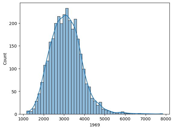
seaborn.histplot(x=pci_df['1969'], kde=True);

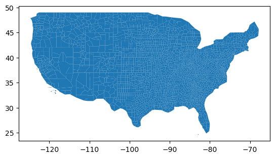
pci_df.plot()
<Axes: >

pci_df = pci_df.to_crs(epsg=5070)
pci_df.plot()
<Axes: >

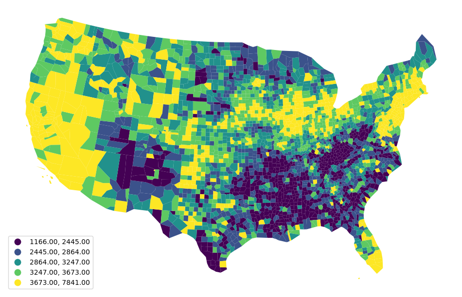
ax = pci_df.plot(
    column='1969',
    scheme='Quantiles',
    legend=True,
    edgecolor="none",
    legend_kwds={"loc": "lower left"},
    figsize=(12, 12),
)
ax.set_axis_off()
plt.show()


top20, bottom20 = pci_df['1969'].quantile([0.8, 0.2])
top20 / bottom20
1.5022494887525562
top20, bottom20
(3673.0, 2445.0)
def ineq_20_20(values):
    top20, bottom20 = values.quantile([0.8, 0.2])
    return top20 / bottom20
import numpy
years = numpy.arange(1969, 2018).astype(str) 
years
array(['1969', '1970', '1971', '1972', '1973', '1974', '1975', '1976',
       '1977', '1978', '1979', '1980', '1981', '1982', '1983', '1984',
       '1985', '1986', '1987', '1988', '1989', '1990', '1991', '1992',
       '1993', '1994', '1995', '1996', '1997', '1998', '1999', '2000',
       '2001', '2002', '2003', '2004', '2005', '2006', '2007', '2008',
       '2009', '2010', '2011', '2012', '2013', '2014', '2015', '2016',
       '2017'], dtype='<U21')
ratio_2020 = pci_df[years].apply(ineq_20_20, axis=0)
ratio_2020.head()
1969    1.502249
1970    1.465717
1971    1.466783
1972    1.462504
1973    1.516387
dtype: float64
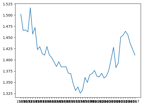
ax = plt.plot(years, ratio_2020)

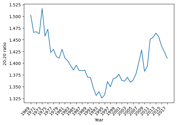
ax = plt.plot(years, ratio_2020)
figure = plt.gcf()
plt.xticks(years[::2])
plt.ylabel("20:20 ratio")
plt.xlabel('Year')
figure.autofmt_xdate(rotation=45)
plt.show()

from pysal.explore import inequality
n = len(pci_df)
n
3076
share_of_population = numpy.arange(1, n+1) / n
share_of_population[0:5]
array([0.0003251 , 0.0006502 , 0.00097529, 0.00130039, 0.00162549])
incomes = pci_df['1969'].sort_values()
shares = incomes / incomes.sum()
shares[0:5]
2647    0.000122
78      0.000130
2981    0.000131
1047    0.000132
973     0.000136
Name: 1969, dtype: float64
cumulative_share = shares.cumsum()
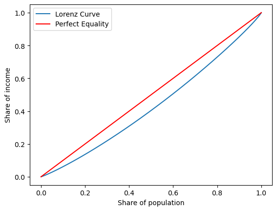
f, ax = plt.subplots()
ax. plot(share_of_population, cumulative_share, label='Lorenz Curve')
ax.plot((0,1), (0,1), color='r', label='Perfect Equality')
ax.set_xlabel("Share of population")
ax.set_ylabel("Share of income")
ax.legend()
plt.show()

g69 = inequality.gini.Gini(pci_df['1969'].values)
g69.g
0.13556175504269904
def gini_by_column(column):
    return inequality.gini.Gini(column.values).g
inequalities = (
    pci_df[years].apply(gini_by_column, axis=0).to_frame("gini")
)
inequalities.head()
gini
1969 0.135562
1970 0.130076
1971 0.128540
1972 0.129126
1973 0.142166
inequalities.plot(figsize=(10,3));

inequalities.head()
gini
1969 0.135562
1970 0.130076
1971 0.128540
1972 0.129126
1973 0.142166
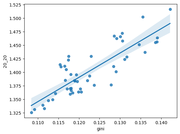
inequalities['20_20'] = ratio_2020
inequalities.head()
gini 20_20
1969 0.135562 1.502249
1970 0.130076 1.465717
1971 0.128540 1.466783
1972 0.129126 1.462504
1973 0.142166 1.516387
_ = seaborn.regplot(x='gini', y='20_20', data=inequalities)