Spatial Autocorrelation Concepts
2/28/23
Outline
- Concepts and Issues
- Null and Alternative Hypotheses
- Spatial Autocorrelation Tests
Concepts and Issues
Spatial Dependence
There is no question with respect to emergent geospatial science. The important harbingers were Geary’s article on spatial autocorrelation, Dacey’s paper about two- and K-color maps, and that of Bachi on geographic series.
– Berry, Griifth, Tiefelsdorf (2008)
Spatial Dependence
Working Concept
what happens at one place depends on events in nearby places
all things are related but nearby things are more related than distant things (Tobler)
central focus in lattice data analysis
Goodchild 1991
a world without positive spatial dependence would be an impossible world
impossible to describe
impossible to live in
hell is a place with no spatial dependence
Spatial Dependence
Categorizing
Type: Substantive versus nuisance
Direction: Positive versus negative
Issues
Time versus space
Inference
Substantive Spatial Dependence
Process Based
Part of the process under study
Leaving it out
Incomplete understanding
Biased inferences
Nuisance Spatial Dependence
Not Process Based
Artifact of data collection
Process boundaries not matching data boundaries
Scattering across pixels
GIS induced
Boundary
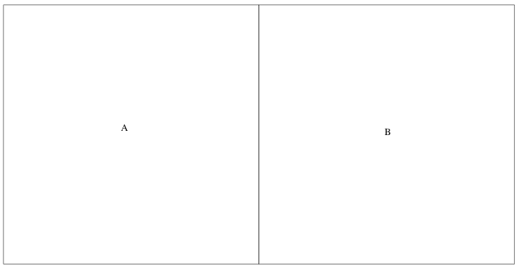
Boundary Mismatch
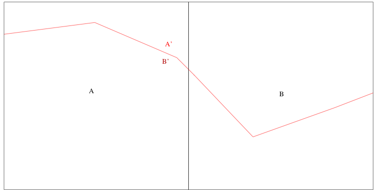
Even if \(A\) and \(B\) are independent
\(A'\) and \(B'\) will be dependent
Nusiance vs. Substantive Dependence
Issues
Not always easy to differentiate from substantive
Different implications for each type
Specification strategies (Econometrics)
Both can be operating jointly
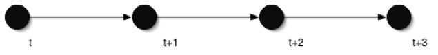
Space versus Time
Temporal Dependence
Past influences the future
Recursive
One dimension
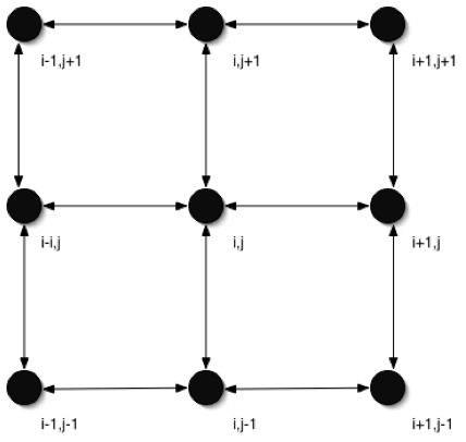
Space versus Time
Spatial Dependence
Multi-directional
Simultaneous
Terminology
Related Concepts
Spatial Dependence
Spatial Autocorrelation
Spatial Association
Spatial Dependence
Distributional Characteristic
Multivariate density function
difficult/impossible to verify empirically
Dependent Distribution
- does not factor in marginal densities
Spatial Autocorrelation
Auto = same variable
Correlation = scaled covariance
Spatial - geographic pattern to the correlation
Spatial Autocorrelation
Measurement of Moment of Distribution
off-diagonal elements of variance-covariance matrix
autocovariance
\(C[y_i,y_j] \ne 0 \ \forall i\ne j\)
can be estimated
Spatial Autocorrelation Coefficient
- significance test on coefficient = 0
Spatial Autocorrelation
Joint multivariate distribution function \[f(y) = \frac{ \exp\left[ -\frac{1}{2} (y-\mu)' \Sigma^{-1} (y-\mu) \right]} {\sqrt{(2\pi)^n|\Sigma|}}\]
Variance-Covariance Matrix
\[\Sigma= \left[ \begin{array}{rrrr} \sigma_{1,1}&\sigma_{1,2}&\ldots&\sigma_{1,n}\\ \sigma_{2,1}&\sigma_{2,2}&\ldots&\sigma_{2,n}\\ \vdots&\vdots&\ddots&\vdots\\ \sigma_{n,1}&\sigma_{n,2}&\ldots&\sigma_{n,n} \end{array} \right]\]
covariance: \(\sigma_{i,j} = E[(y_i - \mu_i)(y_j-\mu_j) ]\)
symmetry: \(\sigma_{i,j} =\sigma_{i,j}\)
variance: \(\sigma_{i,i} = E[(y_i - \mu_i)(y_i-\mu_i) ]\)
Correlation
\[\rho_{ij} = \frac{\sigma_{ij}}{\sqrt{\sigma_{i}^2}\sqrt{\sigma_{j}^2}}\] \[-1.0 \le \rho_{ij} \le 1.0\]
Data Types and Autocorrelation
Point Data
focus on geometric pattern
random vs. nonrandom
clustered vs. uniform
Geostatistics
2-D modeling of spatial covariance (pairs of observations in function of distance)
kriging, spatial prediction
Data Types and Autocorrelation
Lattice Data
areal units: states, counties, census tracts, watersheds
points: centroids of areal units
focus on the spatial nonrandomness of attribute values
Spatial Association
Not a Rigorously Defined Term
Usually the same as spatial autocorrelation
often used in non-technical discussion
avoid unless meaning is clear
Spatial Dependence
Good News (for geographers)
Space matters
Suggestive of underlying process
Bad news
invalidates random sampling assumption
necessitates new methods = spatial statistics and spatial econometrics
Spatial Dependence: Implications
The specific process we are simulating is as follows:\[\begin{aligned} \label{eq:simdgp}y&=&X\beta + \epsilon \\ \nonumber\epsilon &=& \lambda W \epsilon + \nu \end{aligned}\] where \(\nu^{\sim}N(0,\sigma^{2}I)\), \(\lambda\) is a spatial autocorrelation parameter (scalar) and \(W\) is a spatial weights matrix. If \(\lambda=0\) then the \(i.i.d.\) assumption holds, otherwise there is spatial dependence.
\(\beta=40, \ \sigma^2=16, \ x=[1,1,\ldots]\)
\(\lambda=[0.0, 0.25, 0.50, 0.75], \ n=25\)
Spatial Dependence: Implications
For each D.G.P. we are going to generate 500 samples of size \(n=25\) for our map. You can think of this as generating 500 maps using the same D.G.P.. For each sample we will then do the following:
Estimate \(\mu\) with \(\bar{y}\)
Test the hypothesis that \(\mu=40\)
Implications
| \(\lambda\) | 0.00 | 0.25 | 0.50 | 0.75 |
|---|---|---|---|---|
| \(\hat{\mu}\) | 39.947 | 39.931 | 39.901 | 39.814 |
| \(\sigma_{\bar{x}}\) | 0.816 | 1.090 | 1.641 | 3.304 |
| \(p\) | 0.056 | 0.148 | 0.278 | 0.492 |
Null and Alternative Hypotheses
Spatial Randomness
Null Hypothesis
observed spatial pattern of values is equally likely as any other spatial pattern
values at one location do no depend on values at other (neighboring) locations
under spatial randomness, the location of values may be altered without affecting the information content of the data
Spatial Autocorrelation on a Grid
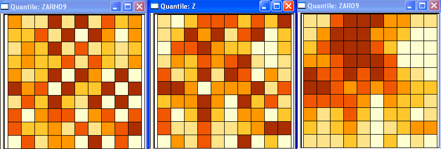
Negative, Random, Positive
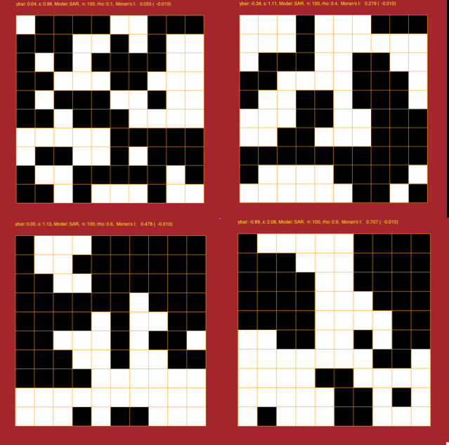
Positive Spatial Autocorrelation
Clustering
- like values tend to be in similar locations
Neighbor similarity
- more alike than they would be under spatial randomness
Compatible with Diffusion
- but not necessarily caused by diffusion
Positive Spatial Autocorrelation
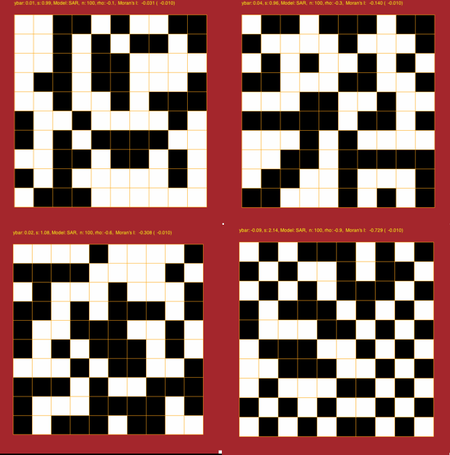
Negative Spatial Autocorrelation
Checkerboard pattern
- anti-clustering
Neighbor dissimilarity
- more dissimilar than they would be under spatial randomness
Compatible with Competition
- but not necessarily caused by competition
Negative Spatial Autocorrelation
Autocorrelation and Diffusion
One does not necessarily imply the other
diffusion tends to yield positive spatial autocorrelation but the reverse is not necessary
positive spatial correlation may be due to structural factors, without contagion or diffusion
True vs. Apparent Contagion
What is the Cause behind the clustering?
True contagion
- result of a contagious process, social interaction, dynamic process
Apparent contagion
spatial heterogeneity
stratification
Cannot be distinguished in a pure cross section
Equifinality or Identification Problem
Spatial Autocorrelation Tests
Clustering
Global characeristic
property of overall pattern = all observations
are like values more grouped in space than random
test by means of a global spatial autocorrelation statistic
no location of the clusters determined
Clusters
Local characeristic
where are the like values more grouped in space than random?
property of local pattern = location-specific
test by means of a local spatial autocorrelation statistic
local clusters may be compatible with global spatial randomness
Spatial Autocorrelation Statistic
Structure
Formal Test of Match between Value Similarity and Locational Similarity
Statistic Summarizes Both Aspects
Significance
- how likely is it (p-value) that the computed statistic would take this (extreme) value in a spatially random pattern
Attribute Similarity
Summary of the similarity or dissimilarity of a variable at different locations
- variable \(y\) at locations \(i,j\) with \(i\ne j\)
Measures of similarity
- cross product: \(y_i y_j\)
Measures of dissimilarity
squared differences: \((y_i - y_j)^2\)
absolute differences: \(|y_i - y_j|\)
Locational Similarity
Formalizing the notion of Neighbor
- when two spatial units a-priori are likely to interact
Spatial Weights
not necessarility geographical
many approaches
Summary
Spatial Dependence
Core of Lattice Analysis
Spatial Autocorrelation More Complex than Temporal Autocorrelation
Combine Value and Locational Similarities